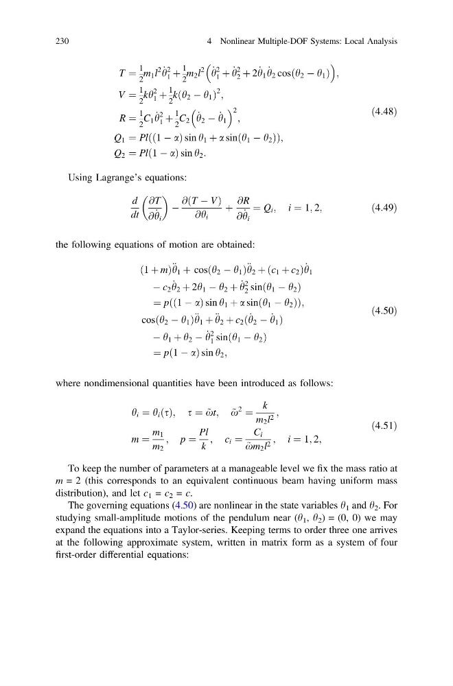
T ¼
1
2
m 1 l
2 _
h
2
1 þ
1
2
m 2 l
2 _
h
2
1 þ _
h
2
2 þ 2 _
h 1 _
h 2 cosðh 2 À h 1 Þ
;
V ¼
1
2
kh
2
1 þ
1
2
k h 2 À h 1
ð
Þ
2 ;
R ¼
1
2
C 1 _
h
2
1 þ
1
2
C 2 _
h 2 À _
h 1
2 ;
Q 1 ¼ Pl ð1 À aÞ sin h 1 þ a sinðh 1 À h 2 Þ
ð
Þ ;
Q 2 ¼ Plð1 À aÞ sin h 2 :
ð4:48Þ
Using Lagrange’s equations:
d
dt
@T
@ _
h i
À
@ T À V
ð
Þ
@h i
þ
@R
@ _
h i
¼ Q i ; i ¼ 1; 2;
ð4:49Þ
the following equations of motion are obtained:
ð1 þ mÞ € h 1 þ cosðh 2 À h 1 Þ € h 2 þ ðc 1 þ c 2 Þ _
h 1
À c 2 _
h 2 þ 2h 1 À h 2 þ _
h
2
2 sinðh 1 À h 2 Þ
¼ p ð1 À aÞ sin h 1 þ a sinðh 1 À h 2 Þ
ð
Þ ;
cosðh 2 À h 1 Þ € h 1 þ € h 2 þ c 2 ð _
h 2 À _
h 1 Þ
À h 1 þ h 2 À _
h
2
1 sinðh 1 À h 2 Þ
¼ pð1 À aÞ sin h 2 ;
ð4:50Þ
where nondimensional quantities have been introduced as follows:
h i ¼ h i ðsÞ; s ¼ ~
xt; ~
x
2
¼
k
m 2 l 2 ;
m ¼
m 1
m 2
; p ¼
Pl
k
; c i ¼
C i
~
xm 2 l 2 ; i ¼ 1; 2;
ð4:51Þ
To keep the number of parameters at a manageable level we fix the mass ratio at
m = 2 (this corresponds to an equivalent continuous beam having uniform mass
distribution), and let c 1 = c 2 = c.
The governing equations (4.50) are nonlinear in the state variables h 1 and h 2 . For
studying small-amplitude motions of the pendulum near (h 1 , h 2 ) = (0, 0) we may
expand the equations into a Taylor-series. Keeping terms to order three one arrives
at the following approximate system, written in matrix form as a system of four
first-order differential equations:
230
4 Nonlinear Multiple-DOF Systems: Local Analysis