

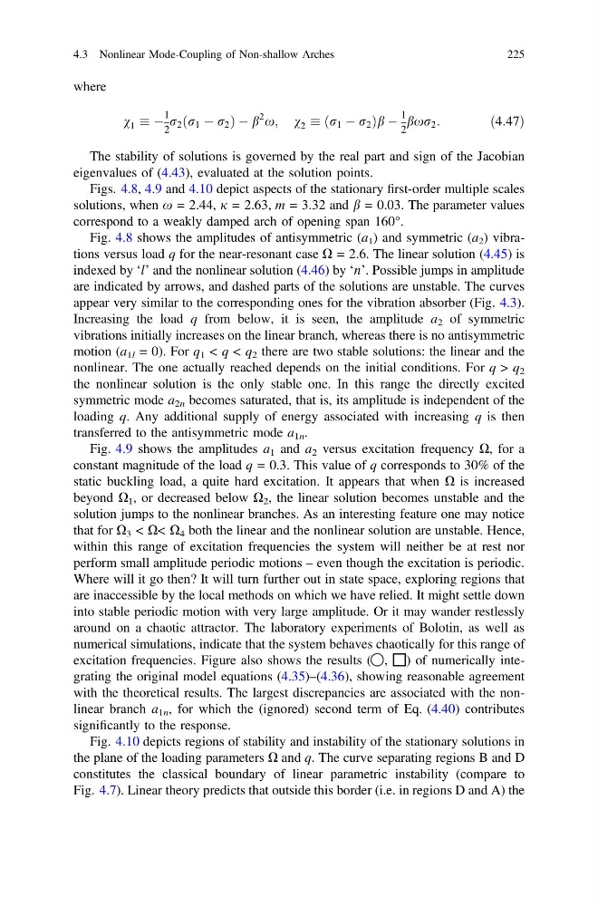
where
v 1 À
1
2
r 2 ðr 1 À r 2 Þ À b
2 x; v 2 ðr 1 À r 2 Þb À
1
2
bxr 2 :
ð4:47Þ
The stability of solutions is governed by the real part and sign of the Jacobian
eigenvalues of (4.43), evaluated at the solution points.
Figs. 4.8, 4.9 and 4.10 depict aspects of the stationary first-order multiple scales
solutions, when x = 2.44, j = 2.63, m = 3.32 and b = 0.03. The parameter values
correspond to a weakly damped arch of opening span 160°.
Fig. 4.8 shows the amplitudes of antisymmetric (a 1 ) and symmetric (a 2 ) vibrations versus load q for the near-resonant case X = 2.6. The linear solution (4.45) is
indexed by ‘l’ and the nonlinear solution (4.46) by ‘n’. Possible jumps in amplitude
are indicated by arrows, and dashed parts of the solutions are unstable. The curves
appear very similar to the corresponding ones for the vibration absorber (Fig. 4.3).
Increasing the load q from below, it is seen, the amplitude a 2 of symmetric
vibrations initially increases on the linear branch, whereas there is no antisymmetric
motion (a 1l = 0). For q 1 < q < q 2 there are two stable solutions: the linear and the
nonlinear. The one actually reached depends on the initial conditions. For q > q 2
the nonlinear solution is the only stable one. In this range the directly excited
symmetric mode a 2n becomes saturated, that is, its amplitude is independent of the
loading q. Any additional supply of energy associated with increasing q is then
transferred to the antisymmetric mode a 1n .
Fig. 4.9 shows the amplitudes a 1 and a 2 versus excitation frequency X, for a
constant magnitude of the load q = 0.3. This value of q corresponds to 30% of the
static buckling load, a quite hard excitation. It appears that when X is increased
beyond X 1 , or decreased below X 2 , the linear solution becomes unstable and the
solution jumps to the nonlinear branches. As an interesting feature one may notice
that for X 3 < X< X 4 both the linear and the nonlinear solution are unstable. Hence,
within this range of excitation frequencies the system will neither be at rest nor
perform small amplitude periodic motions – even though the excitation is periodic.
Where will it go then? It will turn further out in state space, exploring regions that
are inaccessible by the local methods on which we have relied. It might settle down
into stable periodic motion with very large amplitude. Or it may wander restlessly
around on a chaotic attractor. The laboratory experiments of Bolotin, as well as
numerical simulations, indicate that the system behaves chaotically for this range of
excitation frequencies. Figure also shows the results ( ⃝, ⃞) of numerically integrating the original model equations (4.35)–(4.36), showing reasonable agreement
with the theoretical results. The largest discrepancies are associated with the nonlinear branch a 1n , for which the (ignored) second term of Eq. (4.40) contributes
significantly to the response.
Fig. 4.10 depicts regions of stability and instability of the stationary solutions in
the plane of the loading parameters X and q. The curve separating regions B and D
constitutes the classical boundary of linear parametric instability (compare to
Fig. 4.7). Linear theory predicts that outside this border (i.e. in regions D and A) the
4.3 Nonlinear Mode-Coupling of Non-shallow Arches
225
v 1 À
1
2
r 2 ðr 1 À r 2 Þ À b
2 x; v 2 ðr 1 À r 2 Þb À
1
2
bxr 2 :
ð4:47Þ
The stability of solutions is governed by the real part and sign of the Jacobian
eigenvalues of (4.43), evaluated at the solution points.
Figs. 4.8, 4.9 and 4.10 depict aspects of the stationary first-order multiple scales
solutions, when x = 2.44, j = 2.63, m = 3.32 and b = 0.03. The parameter values
correspond to a weakly damped arch of opening span 160°.
Fig. 4.8 shows the amplitudes of antisymmetric (a 1 ) and symmetric (a 2 ) vibrations versus load q for the near-resonant case X = 2.6. The linear solution (4.45) is
indexed by ‘l’ and the nonlinear solution (4.46) by ‘n’. Possible jumps in amplitude
are indicated by arrows, and dashed parts of the solutions are unstable. The curves
appear very similar to the corresponding ones for the vibration absorber (Fig. 4.3).
Increasing the load q from below, it is seen, the amplitude a 2 of symmetric
vibrations initially increases on the linear branch, whereas there is no antisymmetric
motion (a 1l = 0). For q 1 < q < q 2 there are two stable solutions: the linear and the
nonlinear. The one actually reached depends on the initial conditions. For q > q 2
the nonlinear solution is the only stable one. In this range the directly excited
symmetric mode a 2n becomes saturated, that is, its amplitude is independent of the
loading q. Any additional supply of energy associated with increasing q is then
transferred to the antisymmetric mode a 1n .
Fig. 4.9 shows the amplitudes a 1 and a 2 versus excitation frequency X, for a
constant magnitude of the load q = 0.3. This value of q corresponds to 30% of the
static buckling load, a quite hard excitation. It appears that when X is increased
beyond X 1 , or decreased below X 2 , the linear solution becomes unstable and the
solution jumps to the nonlinear branches. As an interesting feature one may notice
that for X 3 < X< X 4 both the linear and the nonlinear solution are unstable. Hence,
within this range of excitation frequencies the system will neither be at rest nor
perform small amplitude periodic motions – even though the excitation is periodic.
Where will it go then? It will turn further out in state space, exploring regions that
are inaccessible by the local methods on which we have relied. It might settle down
into stable periodic motion with very large amplitude. Or it may wander restlessly
around on a chaotic attractor. The laboratory experiments of Bolotin, as well as
numerical simulations, indicate that the system behaves chaotically for this range of
excitation frequencies. Figure also shows the results ( ⃝, ⃞) of numerically integrating the original model equations (4.35)–(4.36), showing reasonable agreement
with the theoretical results. The largest discrepancies are associated with the nonlinear branch a 1n , for which the (ignored) second term of Eq. (4.40) contributes
significantly to the response.
Fig. 4.10 depicts regions of stability and instability of the stationary solutions in
the plane of the loading parameters X and q. The curve separating regions B and D
constitutes the classical boundary of linear parametric instability (compare to
Fig. 4.7). Linear theory predicts that outside this border (i.e. in regions D and A) the
4.3 Nonlinear Mode-Coupling of Non-shallow Arches
225