

zero solution is stable, whereas within the border (regions B and C) it is unstable.
The nonlinear analysis enables us to extend and sharpen the conclusions drawn
from linear analysis, as follows. As for region D, it is correct that the zero solution
is stable. However, the nonlinear (non-zero) solution is stable as well. This means
that the zero solution is stable only to sufficiently small perturbations, since a large
perturbation may carry the system to the stable nonlinear branch. As for region B, it
is correct that the zero solution is unstable. However, this does not mean that the
amplitudes of the system grow without bounds. Rather, they become limited at a
finite value, perhaps very small. As for the knife-shaped region C, the nonlinear
local analysis revealed that no stable periodic motions of small amplitude exist here.
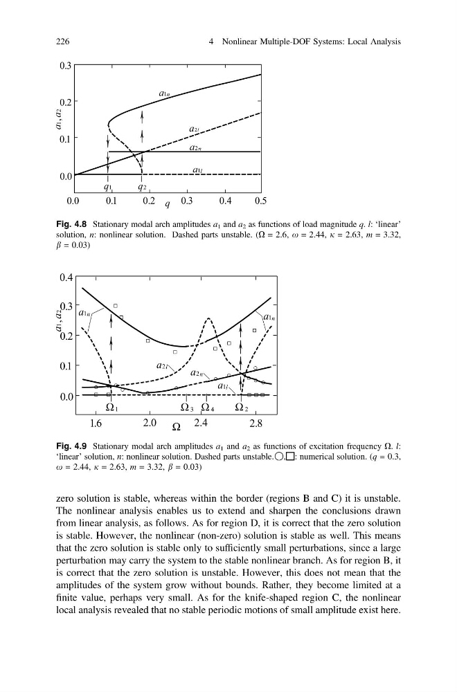
Fig. 4.8 Stationary modal arch amplitudes a 1 and a 2 as functions of load magnitude q. l: ‘linear’
solution, n: nonlinear solution. Dashed parts unstable. (X = 2.6, x = 2.44, j = 2.63, m = 3.32,
b = 0.03)
Fig. 4.9 Stationary modal arch amplitudes a 1 and a 2 as functions of excitation frequency X. l:
‘linear’ solution, n: nonlinear solution. Dashed parts unstable. ⃝, ⃞: numerical solution. (q = 0.3,
x = 2.44, j = 2.63, m = 3.32, b = 0.03)
226
4 Nonlinear Multiple-DOF Systems: Local Analysis
The nonlinear analysis enables us to extend and sharpen the conclusions drawn
from linear analysis, as follows. As for region D, it is correct that the zero solution
is stable. However, the nonlinear (non-zero) solution is stable as well. This means
that the zero solution is stable only to sufficiently small perturbations, since a large
perturbation may carry the system to the stable nonlinear branch. As for region B, it
is correct that the zero solution is unstable. However, this does not mean that the
amplitudes of the system grow without bounds. Rather, they become limited at a
finite value, perhaps very small. As for the knife-shaped region C, the nonlinear
local analysis revealed that no stable periodic motions of small amplitude exist here.
Fig. 4.8 Stationary modal arch amplitudes a 1 and a 2 as functions of load magnitude q. l: ‘linear’
solution, n: nonlinear solution. Dashed parts unstable. (X = 2.6, x = 2.44, j = 2.63, m = 3.32,
b = 0.03)
Fig. 4.9 Stationary modal arch amplitudes a 1 and a 2 as functions of excitation frequency X. l:
‘linear’ solution, n: nonlinear solution. Dashed parts unstable. ⃝, ⃞: numerical solution. (q = 0.3,
x = 2.44, j = 2.63, m = 3.32, b = 0.03)
226
4 Nonlinear Multiple-DOF Systems: Local Analysis