

xðtÞ ¼
Z t
0
FðsÞgðt À sÞ ds;
ð1:11Þ
in which g(t) is the impulse response function:
gðtÞ ¼
1
mx
e
Àfxt
ffiffiffiffiffiffiffiffiffiffiffiffi ffi
1 À f
2
p
sinð ~
xtÞ;
ð1:12Þ
where x, f and ~
x are defined by (1.4), (1.6), and (1.7), respectively.
If the system is not initially at rest, i.e. with non-zero initial conditions, the
homogeneous (freely damped) solution should be added.
1.3 Multiple Degree of Freedom Systems
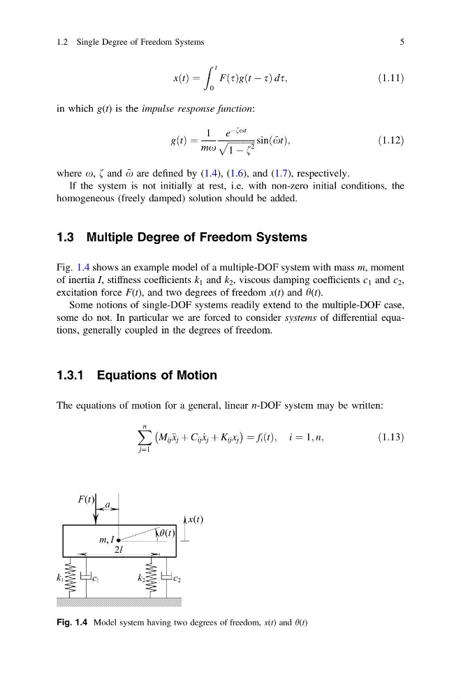
Fig. 1.4 shows an example model of a multiple-DOF system with mass m, moment
of inertia I, stiffness coefficients k 1 and k 2 , viscous damping coefficients c 1 and c 2 ,
excitation force F(t), and two degrees of freedom x(t) and h(t).
Some notions of single-DOF systems readily extend to the multiple-DOF case,
some do not. In particular we are forced to consider systems of differential equations, generally coupled in the degrees of freedom.
1.3.1 Equations of Motion
The equations of motion for a general, linear n-DOF system may be written:
X n
j¼1
M ij € x j þ C ij _
x j þ K ij x j
À
Á ¼ f i ðtÞ; i ¼ 1; n;
ð1:13Þ
Fig. 1.4 Model system having two degrees of freedom, x(t) and h(t)
1.2 Single Degree of Freedom Systems
5
Z t
0
FðsÞgðt À sÞ ds;
ð1:11Þ
in which g(t) is the impulse response function:
gðtÞ ¼
1
mx
e
Àfxt
ffiffiffiffiffiffiffiffiffiffiffiffi ffi
1 À f
2
p
sinð ~
xtÞ;
ð1:12Þ
where x, f and ~
x are defined by (1.4), (1.6), and (1.7), respectively.
If the system is not initially at rest, i.e. with non-zero initial conditions, the
homogeneous (freely damped) solution should be added.
1.3 Multiple Degree of Freedom Systems
Fig. 1.4 shows an example model of a multiple-DOF system with mass m, moment
of inertia I, stiffness coefficients k 1 and k 2 , viscous damping coefficients c 1 and c 2 ,
excitation force F(t), and two degrees of freedom x(t) and h(t).
Some notions of single-DOF systems readily extend to the multiple-DOF case,
some do not. In particular we are forced to consider systems of differential equations, generally coupled in the degrees of freedom.
1.3.1 Equations of Motion
The equations of motion for a general, linear n-DOF system may be written:
X n
j¼1
M ij € x j þ C ij _
x j þ K ij x j
À
Á ¼ f i ðtÞ; i ¼ 1; n;
ð1:13Þ
Fig. 1.4 Model system having two degrees of freedom, x(t) and h(t)
1.2 Single Degree of Freedom Systems
5