

where
H ¼
F 0
ffiffiffiffiffiffiffiffiffiffiffiffiffiffiffiffiffiffiffiffiffiffiffiffiffiffiffiffiffiffiffiffiffiffiffiffiffiffiffiffi
k À mX
2
À
Á 2 þ cX
ð Þ
2
q
; tan u ¼
cX
k À mX
2
:
ð1:9Þ
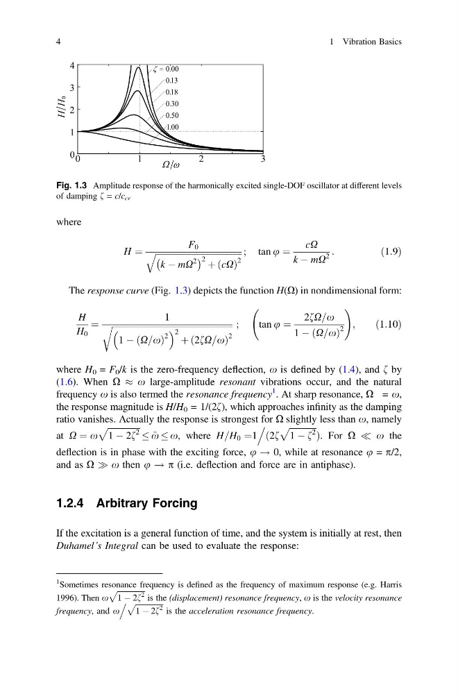
The response curve (Fig. 1.3) depicts the function H(X) in nondimensional form:
H
H 0
¼
1
ffiffiffiffiffiffiffiffiffiffiffiffiffiffiffiffiffiffiffiffiffiffiffiffiffiffiffiffiffiffiffiffiffiffiffiffiffiffiffiffiffiffiffiffiffiffiffiffiffiffiffiffiffiffiffiffi
1 À ðX=xÞ
2
2 þ 2fX=x
ð
Þ
2
r
;
tan u ¼
2fX=x
1 À ðX=xÞ
2
!
;
ð1:10Þ
where H 0 = F 0 /k is the zero-frequency deflection, x is defined by (1.4), and f by
(1.6). When X % x large-amplitude resonant vibrations occur, and the natural
frequency x is also termed the resonance frequency
1 . At sharp resonance, X = x,
the response magnitude is H/H 0 = 1/(2f), which approaches infinity as the damping
ratio vanishes. Actually the response is strongest for X slightly less than x, namely
at X ¼ x
ffiffiffiffiffiffiffiffiffiffiffiffiffiffiffi
1 À 2f
2
p
~
x x, where H=H 0 ¼1
.
ð2f
ffiffiffiffiffiffiffiffiffiffiffiffi ffi
1 À f
2
p
Þ. For X ( x the
deflection is in phase with the exciting force, u ! 0, while at resonance u = p/2,
and as X ) x then u ! p (i.e. deflection and force are in antiphase).
1.2.4 Arbitrary Forcing
If the excitation is a general function of time, and the system is initially at rest, then
Duhamel’s Integral can be used to evaluate the response:
Fig. 1.3 Amplitude response of the harmonically excited single-DOF oscillator at different levels
of damping f = c/c cr
1
Sometimes resonance frequency is defined as the frequency of maximum response (e.g. Harris
1996). Then x
ffiffiffiffiffiffiffiffiffiffiffiffiffiffiffi
1 À 2f
2
p
is the (displacement) resonance frequency, x is the velocity resonance
frequency, and x
. ffiffiffiffiffiffiffiffiffiffiffiffiffiffiffi
1 À 2f
2
p
is the acceleration resonance frequency.
4
1 Vibration Basics
H ¼
F 0
ffiffiffiffiffiffiffiffiffiffiffiffiffiffiffiffiffiffiffiffiffiffiffiffiffiffiffiffiffiffiffiffiffiffiffiffiffiffiffiffi
k À mX
2
À
Á 2 þ cX
ð Þ
2
q
; tan u ¼
cX
k À mX
2
:
ð1:9Þ
The response curve (Fig. 1.3) depicts the function H(X) in nondimensional form:
H
H 0
¼
1
ffiffiffiffiffiffiffiffiffiffiffiffiffiffiffiffiffiffiffiffiffiffiffiffiffiffiffiffiffiffiffiffiffiffiffiffiffiffiffiffiffiffiffiffiffiffiffiffiffiffiffiffiffiffiffiffi
1 À ðX=xÞ
2
2 þ 2fX=x
ð
Þ
2
r
;
tan u ¼
2fX=x
1 À ðX=xÞ
2
!
;
ð1:10Þ
where H 0 = F 0 /k is the zero-frequency deflection, x is defined by (1.4), and f by
(1.6). When X % x large-amplitude resonant vibrations occur, and the natural
frequency x is also termed the resonance frequency
1 . At sharp resonance, X = x,
the response magnitude is H/H 0 = 1/(2f), which approaches infinity as the damping
ratio vanishes. Actually the response is strongest for X slightly less than x, namely
at X ¼ x
ffiffiffiffiffiffiffiffiffiffiffiffiffiffiffi
1 À 2f
2
p
~
x x, where H=H 0 ¼1
.
ð2f
ffiffiffiffiffiffiffiffiffiffiffiffi ffi
1 À f
2
p
Þ. For X ( x the
deflection is in phase with the exciting force, u ! 0, while at resonance u = p/2,
and as X ) x then u ! p (i.e. deflection and force are in antiphase).
1.2.4 Arbitrary Forcing
If the excitation is a general function of time, and the system is initially at rest, then
Duhamel’s Integral can be used to evaluate the response:
Fig. 1.3 Amplitude response of the harmonically excited single-DOF oscillator at different levels
of damping f = c/c cr
1
Sometimes resonance frequency is defined as the frequency of maximum response (e.g. Harris
1996). Then x
ffiffiffiffiffiffiffiffiffiffiffiffiffiffiffi
1 À 2f
2
p
is the (displacement) resonance frequency, x is the velocity resonance
frequency, and x
. ffiffiffiffiffiffiffiffiffiffiffiffiffiffiffi
1 À 2f
2
p
is the acceleration resonance frequency.
4
1 Vibration Basics