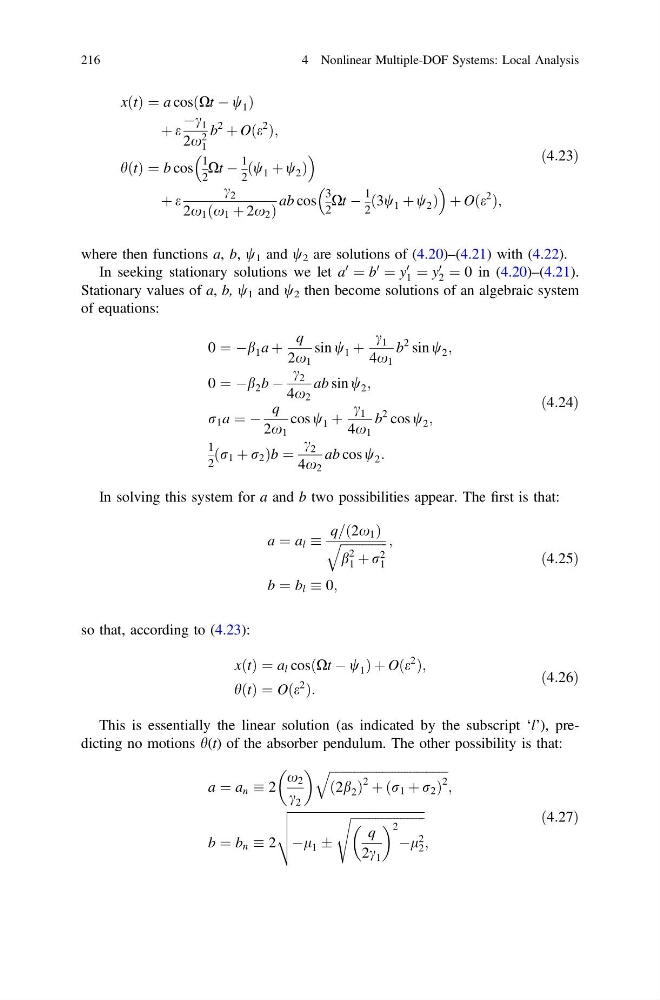
xðtÞ ¼ a cos Xt À w 1
ð
Þ
þ e
Àc 1
2x 2
1
b
2
þ Oðe
2
Þ;
hðtÞ ¼ b cos
1
2
Xt À
1
2
ðw 1 þ w 2 Þ
þ e
c 2
2x 1 ðx 1 þ 2x 2 Þ
ab cos
3
2
Xt À
1
2
3w 1 þ w 2
ð
Þ
þ Oðe
2
Þ;
ð4:23Þ
where then functions a, b, w 1 and w 2 are solutions of (4.20)–(4.21) with (4.22).
In seeking stationary solutions we let a
0
¼ b
0
¼ y
0
1 ¼ y
0
2 ¼ 0 in (4.20)–(4.21).
Stationary values of a, b, w 1 and w 2 then become solutions of an algebraic system
of equations:
0 ¼ Àb 1 a þ
q
2x 1
sin w 1 þ
c 1
4x 1
b
2 sin w 2 ;
0 ¼ Àb 2 b À
c 2
4x 2
ab sin w 2 ;
r 1 a ¼ À
q
2x 1
cos w 1 þ
c 1
4x 1
b
2 cos w 2 ;
1
2
ðr 1 þ r 2 Þb ¼
c 2
4x 2
ab cos w 2 :
ð4:24Þ
In solving this system for a and b two possibilities appear. The first is that:
a ¼ a l
q=ð2x 1 Þ
ffiffiffiffiffiffiffiffiffiffiffiffiffiffi ffi
b
2
1 þ r 2
1
q
;
b ¼ b l 0;
ð4:25Þ
so that, according to (4.23):
xðtÞ ¼ a l cos Xt À w 1
ð
ÞþOðe
2
Þ;
hðtÞ ¼ Oðe
2
Þ:
ð4:26Þ
This is essentially the linear solution (as indicated by the subscript ‘l’), predicting no motions h(t) of the absorber pendulum. The other possibility is that:
a ¼ a n 2
x 2
c 2
ffiffiffiffiffiffiffiffiffiffiffiffiffiffiffiffiffiffiffiffiffiffiffiffiffiffiffiffiffiffiffiffiffiffiffiffiffiffi
2b 2
ð Þ
2 þ r 1 þ r 2
ð
Þ
2
q
;
b ¼ b n 2
ffiffiffiffiffiffiffiffiffiffiffiffiffiffiffiffiffiffiffiffiffiffiffiffiffiffiffiffiffiffiffiffiffiffiffiffiffiffiffiffiffiffiffi
Àl 1 Æ
ffiffiffiffiffiffiffiffiffiffiffiffiffiffiffiffiffiffiffiffiffiffiffiffi
q
2c 1
2
Àl 2
2
s
v
u
u
t
;
ð4:27Þ
216
4 Nonlinear Multiple-DOF Systems: Local Analysis