

3.9.5 Example 3: Self-excited Friction Oscillator
with a One-Sided Stop
Fig. 3.32(a) shows the classical ‘mass on moving belt’ model (Panovko and
Gubanova 1965), though extended with a stop at the right, which restricts motions
to s < D (the left stop is ignored in this section but included in the following
Sect. 3.9.6). Without stop(s) this system is often used for illustrating
friction-induced oscillation, e.g., Thomsen and Fidlin (2003) used averaging to
derive stationary amplitudes for pure slip and stick–slip oscillations. With stop(s),
the system models rubbing objects with slipping parts, e.g., loosely mounted brake
pads.
A typical nondimensional model formulation of the equations of motion is:
€ s þ s ¼ Àh _
s
ð Þ for s \D; _
s\v b ;
s þ ¼ s À ; _
s þ ¼ ÀR_ s À for s ¼ D;
ð3:283Þ
where s(t) is the displacement of the mass from the static equilibrium s 0 = l(–v b ) at
belt speed v b , R is the coefficient of impact restitution, and the friction law is a cubic
Stribeck model with friction coefficient l(v r ) = l s sgn(v r ) – k 1 v r + k 3 v r
3 depending
on relative interface velocity v r ¼ _
s À v b (Ibrahim 1992b; Thomsen and Fidlin
2003, and Fig. 3.32(b)). Here l s is the static coefficient of friction, k 1 the slope of
the friction-velocity curve at zero relative velocity, k 3 the coefficient governing
increased friction at higher velocities. The dissipation function h in (3.283) is then:
h _
s
ð Þ ¼ h 1 _
s þ h 2 _
s
2
þ h 3 _
s
3
;
ð3:284Þ
where h 1 = 2b– k 1 + 3k 3 v b
2 < 0, h 2 = –3k 3b , h 3 = k, and b is the linear viscous
damping ratio. Of interest here is the effect of impacts, so _
s\v b (i.e. v r < 0) is
assumed to avoid unnecessary complications connected with sticking motions
(stick-slip is considered in Thomsen and Fidlin 2003).
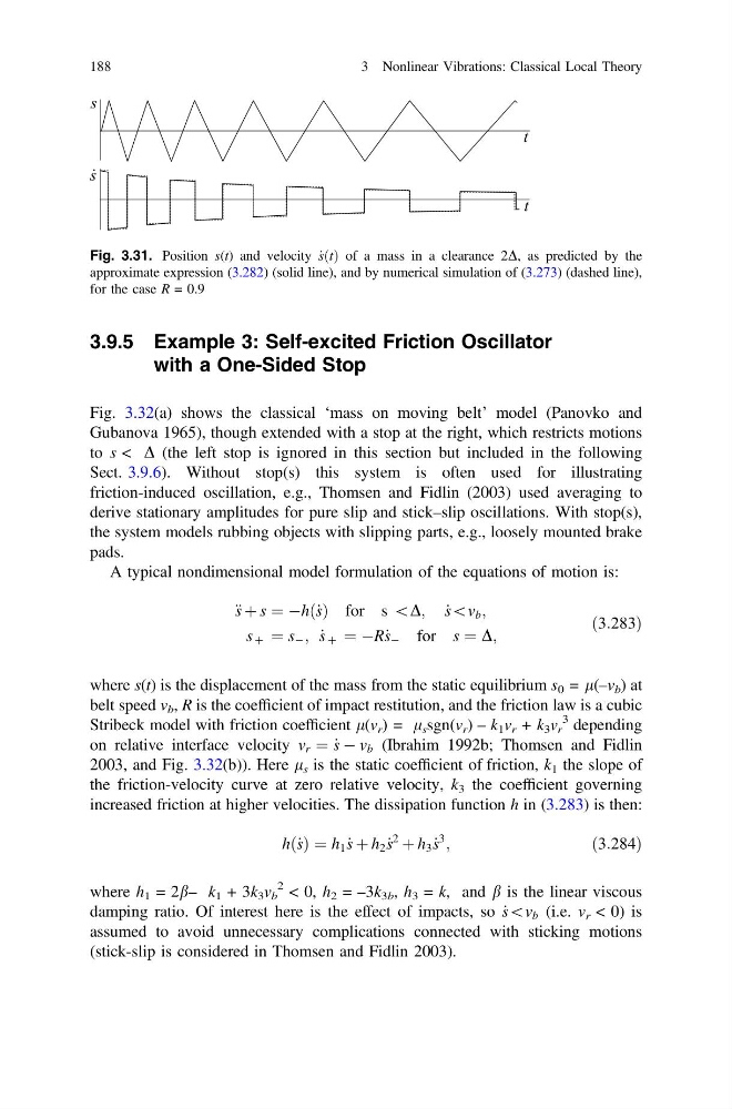
Fig. 3.31. Position s(t) and velocity _
sðtÞ of a mass in a clearance 2D, as predicted by the
approximate expression (3.282) (solid line), and by numerical simulation of (3.273) (dashed line),
for the case R = 0.9
188
3 Nonlinear Vibrations: Classical Local Theory
with a One-Sided Stop
Fig. 3.32(a) shows the classical ‘mass on moving belt’ model (Panovko and
Gubanova 1965), though extended with a stop at the right, which restricts motions
to s < D (the left stop is ignored in this section but included in the following
Sect. 3.9.6). Without stop(s) this system is often used for illustrating
friction-induced oscillation, e.g., Thomsen and Fidlin (2003) used averaging to
derive stationary amplitudes for pure slip and stick–slip oscillations. With stop(s),
the system models rubbing objects with slipping parts, e.g., loosely mounted brake
pads.
A typical nondimensional model formulation of the equations of motion is:
€ s þ s ¼ Àh _
s
ð Þ for s \D; _
s\v b ;
s þ ¼ s À ; _
s þ ¼ ÀR_ s À for s ¼ D;
ð3:283Þ
where s(t) is the displacement of the mass from the static equilibrium s 0 = l(–v b ) at
belt speed v b , R is the coefficient of impact restitution, and the friction law is a cubic
Stribeck model with friction coefficient l(v r ) = l s sgn(v r ) – k 1 v r + k 3 v r
3 depending
on relative interface velocity v r ¼ _
s À v b (Ibrahim 1992b; Thomsen and Fidlin
2003, and Fig. 3.32(b)). Here l s is the static coefficient of friction, k 1 the slope of
the friction-velocity curve at zero relative velocity, k 3 the coefficient governing
increased friction at higher velocities. The dissipation function h in (3.283) is then:
h _
s
ð Þ ¼ h 1 _
s þ h 2 _
s
2
þ h 3 _
s
3
;
ð3:284Þ
where h 1 = 2b– k 1 + 3k 3 v b
2 < 0, h 2 = –3k 3b , h 3 = k, and b is the linear viscous
damping ratio. Of interest here is the effect of impacts, so _
s\v b (i.e. v r < 0) is
assumed to avoid unnecessary complications connected with sticking motions
(stick-slip is considered in Thomsen and Fidlin 2003).
Fig. 3.31. Position s(t) and velocity _
sðtÞ of a mass in a clearance 2D, as predicted by the
approximate expression (3.282) (solid line), and by numerical simulation of (3.273) (dashed line),
for the case R = 0.9
188
3 Nonlinear Vibrations: Classical Local Theory