

or, eliminating time as the independent variable by dividing the second equation
with the first:
dv
dz
¼ 0 for z 6 ¼
p
2
þ jp;
v þ À v À ¼ À 1 À R
ð
Þv À for z ¼
p
2
þ jp;
ð3:279Þ
where instead z now takes the role of the independent variable. This system has the
general form (3.258), and can thus be averaged using (3.259) into:
dv 1
dz 1
¼ À
1 À R
p
v 1 ; v 1 ¼
dz 1
dt
;
ð3:280Þ
which is a linear system with solution:
z 1 ¼
p
1 À R
ln C 1 t þ C 2
ð
Þ ; v 1 ¼
p
1 À R
C 1
C 1 t þ C 2
;
ð3:281Þ
where the constants C 1 > 0 and C 2 are determined by initial conditions. The corresponding motion in terms of the original variable s(t) is then, by (3.275):
s ¼
2D
p
P
p
1 À R
ln C 1 t þ C 2
ð
Þ
:
ð3:282Þ
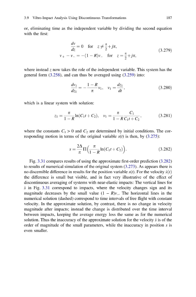
Fig. 3.31 compares results of using the approximate first-order prediction (3.282)
to results of numerical simulation of the original system (3.273). As appears there is
no discernible difference in results for the position variable s(t). For the velocity _
sðtÞ
the difference is small but visible, and in fact very illustrative of the effect of
discontinuous averaging of systems with near-elastic impacts: The vertical lines for
_
s in Fig. 3.31 correspond to impacts, where the velocity changes sign and its
magnitude decreases by the small value (1 – R)v – . The horizontal lines in the
numerical solution (dashed) correspond to time intervals of free flight with constant
velocity. In the approximate solution, by contrast, there is no change in velocity
magnitude after impacts; instead the change is distributed over the time interval
between impacts, keeping the average energy loss the same as for the numerical
solution. Thus the inaccuracy of the approximate solution for the velocity _
s is of the
order of magnitude of the small parameters, while the inaccuracy in position s is
even smaller.
3.9 Vibro-Impact Analysis Using Discontinuous Transformations
187
with the first:
dv
dz
¼ 0 for z 6 ¼
p
2
þ jp;
v þ À v À ¼ À 1 À R
ð
Þv À for z ¼
p
2
þ jp;
ð3:279Þ
where instead z now takes the role of the independent variable. This system has the
general form (3.258), and can thus be averaged using (3.259) into:
dv 1
dz 1
¼ À
1 À R
p
v 1 ; v 1 ¼
dz 1
dt
;
ð3:280Þ
which is a linear system with solution:
z 1 ¼
p
1 À R
ln C 1 t þ C 2
ð
Þ ; v 1 ¼
p
1 À R
C 1
C 1 t þ C 2
;
ð3:281Þ
where the constants C 1 > 0 and C 2 are determined by initial conditions. The corresponding motion in terms of the original variable s(t) is then, by (3.275):
s ¼
2D
p
P
p
1 À R
ln C 1 t þ C 2
ð
Þ
:
ð3:282Þ
Fig. 3.31 compares results of using the approximate first-order prediction (3.282)
to results of numerical simulation of the original system (3.273). As appears there is
no discernible difference in results for the position variable s(t). For the velocity _
sðtÞ
the difference is small but visible, and in fact very illustrative of the effect of
discontinuous averaging of systems with near-elastic impacts: The vertical lines for
_
s in Fig. 3.31 correspond to impacts, where the velocity changes sign and its
magnitude decreases by the small value (1 – R)v – . The horizontal lines in the
numerical solution (dashed) correspond to time intervals of free flight with constant
velocity. In the approximate solution, by contrast, there is no change in velocity
magnitude after impacts; instead the change is distributed over the time interval
between impacts, keeping the average energy loss the same as for the numerical
solution. Thus the inaccuracy of the approximate solution for the velocity _
s is of the
order of magnitude of the small parameters, while the inaccuracy in position s is
even smaller.
3.9 Vibro-Impact Analysis Using Discontinuous Transformations
187