

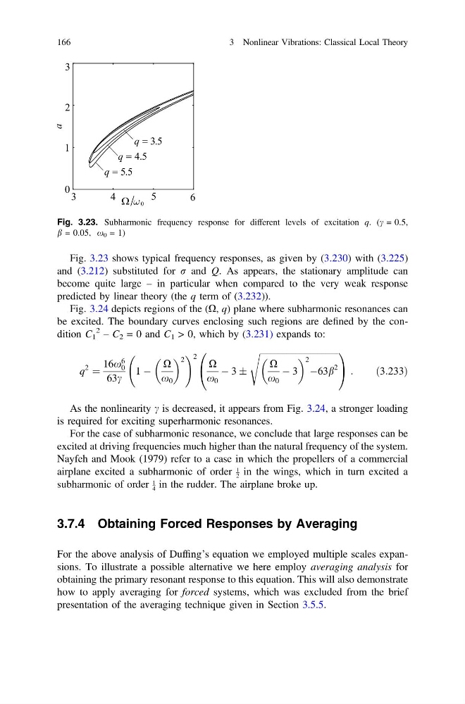
Fig. 3.23 shows typical frequency responses, as given by (3.230) with (3.225)
and (3.212) substituted for r and Q. As appears, the stationary amplitude can
become quite large – in particular when compared to the very weak response
predicted by linear theory (the q term of (3.232)).
Fig. 3.24 depicts regions of the (X, q) plane where subharmonic resonances can
be excited. The boundary curves enclosing such regions are defined by the condition C 1
2
– C 2 = 0 and C 1 > 0, which by (3.231) expands to:
q
2
¼
16x
6
0
63c
1 À
X
x 0
2
! 2 X
x 0
À 3 Æ
ffiffiffiffiffiffiffiffiffiffiffiffiffiffiffiffiffiffiffiffiffiffiffiffiffiffiffiffiffiffiffiffiffiffiffiffi
X
x 0
À 3
2
À63b
2
s
0
@
1
A :
ð3:233Þ
As the nonlinearity c is decreased, it appears from Fig. 3.24, a stronger loading
is required for exciting superharmonic resonances.
For the case of subharmonic resonance, we conclude that large responses can be
excited at driving frequencies much higher than the natural frequency of the system.
Nayfeh and Mook (1979) refer to a case in which the propellers of a commercial
airplane excited a subharmonic of order
1
2 in the wings, which in turn excited a
subharmonic of order
1
4 in the rudder. The airplane broke up.
3.7.4 Obtaining Forced Responses by Averaging
For the above analysis of Duffing’s equation we employed multiple scales expansions. To illustrate a possible alternative we here employ averaging analysis for
obtaining the primary resonant response to this equation. This will also demonstrate
how to apply averaging for forced systems, which was excluded from the brief
presentation of the averaging technique given in Section 3.5.5.
Fig. 3.23. Subharmonic frequency response for different levels of excitation q. (c = 0.5,
b = 0.05, x 0 = 1)
166
3 Nonlinear Vibrations: Classical Local Theory
and (3.212) substituted for r and Q. As appears, the stationary amplitude can
become quite large – in particular when compared to the very weak response
predicted by linear theory (the q term of (3.232)).
Fig. 3.24 depicts regions of the (X, q) plane where subharmonic resonances can
be excited. The boundary curves enclosing such regions are defined by the condition C 1
2
– C 2 = 0 and C 1 > 0, which by (3.231) expands to:
q
2
¼
16x
6
0
63c
1 À
X
x 0
2
! 2 X
x 0
À 3 Æ
ffiffiffiffiffiffiffiffiffiffiffiffiffiffiffiffiffiffiffiffiffiffiffiffiffiffiffiffiffiffiffiffiffiffiffiffi
X
x 0
À 3
2
À63b
2
s
0
@
1
A :
ð3:233Þ
As the nonlinearity c is decreased, it appears from Fig. 3.24, a stronger loading
is required for exciting superharmonic resonances.
For the case of subharmonic resonance, we conclude that large responses can be
excited at driving frequencies much higher than the natural frequency of the system.
Nayfeh and Mook (1979) refer to a case in which the propellers of a commercial
airplane excited a subharmonic of order
1
2 in the wings, which in turn excited a
subharmonic of order
1
4 in the rudder. The airplane broke up.
3.7.4 Obtaining Forced Responses by Averaging
For the above analysis of Duffing’s equation we employed multiple scales expansions. To illustrate a possible alternative we here employ averaging analysis for
obtaining the primary resonant response to this equation. This will also demonstrate
how to apply averaging for forced systems, which was excluded from the brief
presentation of the averaging technique given in Section 3.5.5.
Fig. 3.23. Subharmonic frequency response for different levels of excitation q. (c = 0.5,
b = 0.05, x 0 = 1)
166
3 Nonlinear Vibrations: Classical Local Theory