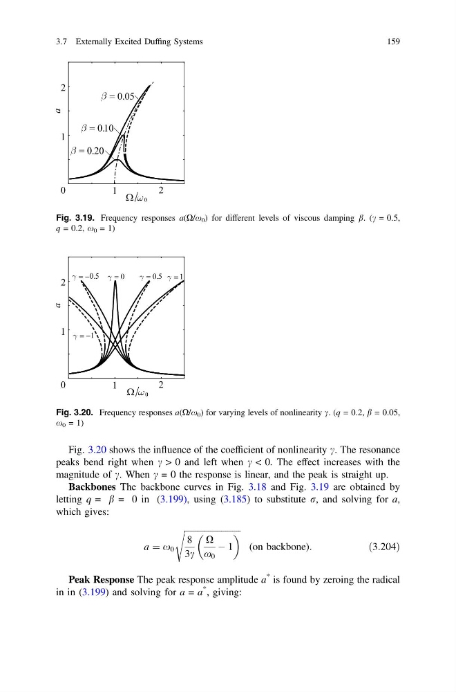
Fig. 3.20 shows the influence of the coefficient of nonlinearity c. The resonance
peaks bend right when c > 0 and left when c < 0. The effect increases with the
magnitude of c. When c = 0 the response is linear, and the peak is straight up.
Backbones The backbone curves in Fig. 3.18 and Fig. 3.19 are obtained by
letting q = b = 0 in (3.199), using (3.185) to substitute r, and solving for a,
which gives:
a ¼ x 0
ffiffiffiffiffiffiffiffiffiffiffiffiffiffiffiffiffiffiffiffiffiffiffiffiffiffi
8
3c
X
x 0
À 1
s
(on backbone):
ð3:204Þ
Peak Response The peak response amplitude a
* is found by zeroing the radical
in in (3.199) and solving for a = a
* , giving:
Fig. 3.19. Frequency responses a(X/x 0 ) for different levels of viscous damping b. (c = 0.5,
q = 0.2, x 0 = 1)
Fig. 3.20. Frequency responses a(X/x 0 ) for varying levels of nonlinearity c. (q = 0.2, b = 0.05,
x 0 = 1)
3.7 Externally Excited Duffing Systems
159