

where the singular points ~ a and ~
w are given by the solutions to (3.194) and (3.195).
Using (3.193) with a′ = w′ = 0 to eliminate cos ~
w and sin ~
w, we obtain:
Jð~ a; ~
wÞ ¼
Àbx 0
À r~ a À
3c
8x 0
~ a
3
1
~ a 2 r~ a À
9c
8x 0
~ a
3
Àbx 0
2
4
3
5 :
ð3:201Þ
Computing eigenvalues as the solutions of |J(~ a, ~
w) – kI| = 0 it is found that:
k ¼ Àbx 0 Æ
ffiffiffiffiffiffiffiffiffiffiffiffiffiffiffiffiffiffiffiffiffiffiffiffiffiffiffiffiffiffiffiffiffiffiffiffiffiffiffiffiffiffiffiffiffiffiffiffiffiffiffiffiffiffiffiffiffiffiffiffi ffi
À r À
3c
8x 0
~ a 2
r À
9c
8x 0
~ a 2
s
:
ð3:202Þ
A solution ~ a is unstable if at least one eigenvalue has a positive real part,
otherwise it is stable. Hence, for ~ a to be unstable it is required that:
r À
3c
8x 0
~ a
2
r À
9c
8x 0
~ a
2
þ bx 0
ð
Þ
2 \0:
ð3:203Þ
This condition is met on the part A-C of the frequency response in Fig. 3.17,
which is thus unstable and drawn in dashed line. All other parts of the response are
stable.
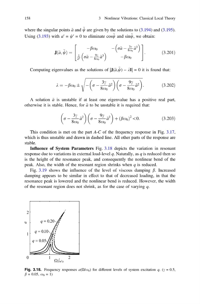
Influence of System Parameters Fig. 3.18 depicts the variation in resonant
response due to variations in external load-level q. Naturally, as q is reduced then so
is the height of the resonance peak, and consequently the nonlinear bend of the
peak. Also, the width of the resonant region shrinks when q is reduced.
Fig. 3.19 shows the influence of the level of viscous damping b. Increased
damping appears to be similar in effect to that of decreased loading, in that the
resonance peak is lowered and the nonlinear bend is reduced. However, the width
of the resonant region does not shrink, as for the case of varying q.
Fig. 3.18. Frequency responses a(X/x 0 ) for different levels of system excitation q. (c = 0.5,
b = 0.05, x 0 = 1)
158
3 Nonlinear Vibrations: Classical Local Theory
w are given by the solutions to (3.194) and (3.195).
Using (3.193) with a′ = w′ = 0 to eliminate cos ~
w and sin ~
w, we obtain:
Jð~ a; ~
wÞ ¼
Àbx 0
À r~ a À
3c
8x 0
~ a
3
1
~ a 2 r~ a À
9c
8x 0
~ a
3
Àbx 0
2
4
3
5 :
ð3:201Þ
Computing eigenvalues as the solutions of |J(~ a, ~
w) – kI| = 0 it is found that:
k ¼ Àbx 0 Æ
ffiffiffiffiffiffiffiffiffiffiffiffiffiffiffiffiffiffiffiffiffiffiffiffiffiffiffiffiffiffiffiffiffiffiffiffiffiffiffiffiffiffiffiffiffiffiffiffiffiffiffiffiffiffiffiffiffiffiffiffi ffi
À r À
3c
8x 0
~ a 2
r À
9c
8x 0
~ a 2
s
:
ð3:202Þ
A solution ~ a is unstable if at least one eigenvalue has a positive real part,
otherwise it is stable. Hence, for ~ a to be unstable it is required that:
r À
3c
8x 0
~ a
2
r À
9c
8x 0
~ a
2
þ bx 0
ð
Þ
2 \0:
ð3:203Þ
This condition is met on the part A-C of the frequency response in Fig. 3.17,
which is thus unstable and drawn in dashed line. All other parts of the response are
stable.
Influence of System Parameters Fig. 3.18 depicts the variation in resonant
response due to variations in external load-level q. Naturally, as q is reduced then so
is the height of the resonance peak, and consequently the nonlinear bend of the
peak. Also, the width of the resonant region shrinks when q is reduced.
Fig. 3.19 shows the influence of the level of viscous damping b. Increased
damping appears to be similar in effect to that of decreased loading, in that the
resonance peak is lowered and the nonlinear bend is reduced. However, the width
of the resonant region does not shrink, as for the case of varying q.
Fig. 3.18. Frequency responses a(X/x 0 ) for different levels of system excitation q. (c = 0.5,
b = 0.05, x 0 = 1)
158
3 Nonlinear Vibrations: Classical Local Theory