

in a
2 . Instead we compute data for the response curves by considering X, rather
than a, as the dependent variable. Inserting r = X – x 0 into (3.194) and solving for
X, we obtain the response curves in the form X(a), as follows:
X
x 0
¼ 1 þ
3c
8x 2
0
a
2
Æ
ffiffiffiffiffiffiffiffiffiffiffiffiffiffiffiffiffiffiffiffiffiffiffiffiffiffiffi ffi
q
2x 2
0 a
2
Àb
2
s
:
ð3:199Þ
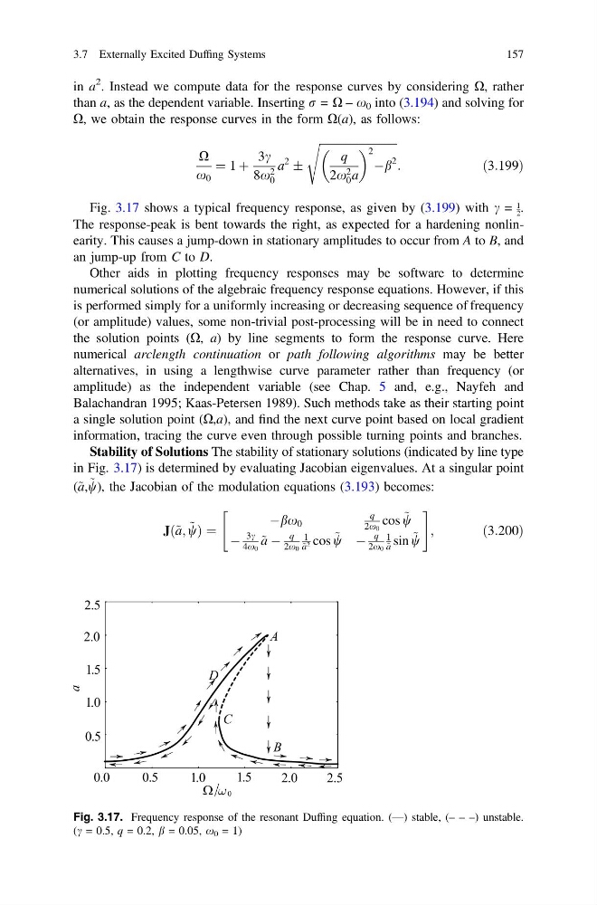
Fig. 3.17 shows a typical frequency response, as given by (3.199) with c =
1
2 .
The response-peak is bent towards the right, as expected for a hardening nonlinearity. This causes a jump-down in stationary amplitudes to occur from A to B, and
an jump-up from C to D.
Other aids in plotting frequency responses may be software to determine
numerical solutions of the algebraic frequency response equations. However, if this
is performed simply for a uniformly increasing or decreasing sequence of frequency
(or amplitude) values, some non-trivial post-processing will be in need to connect
the solution points (X, a) by line segments to form the response curve. Here
numerical arclength continuation or path following algorithms may be better
alternatives, in using a lengthwise curve parameter rather than frequency (or
amplitude) as the independent variable (see Chap. 5 and, e.g., Nayfeh and
Balachandran 1995; Kaas-Petersen 1989). Such methods take as their starting point
a single solution point (X,a), and find the next curve point based on local gradient
information, tracing the curve even through possible turning points and branches.
Stability of Solutions The stability of stationary solutions (indicated by line type
in Fig. 3.17) is determined by evaluating Jacobian eigenvalues. At a singular point
(~ a, ~
w), the Jacobian of the modulation equations (3.193) becomes:
Jð~ a; ~
wÞ ¼
Àbx 0
q
2x 0
cos ~
w
À
3c
4x 0
~ a À
q
2x 0
1
~ a 2 cos ~
w À
q
2x 0
1
~ a sin ~
w
"
#
;
ð3:200Þ
Fig. 3.17. Frequency response of the resonant Duffing equation. (—) stable, (– – –) unstable.
(c = 0.5, q = 0.2, b = 0.05, x 0 = 1)
3.7 Externally Excited Duffing Systems
157
2 . Instead we compute data for the response curves by considering X, rather
than a, as the dependent variable. Inserting r = X – x 0 into (3.194) and solving for
X, we obtain the response curves in the form X(a), as follows:
X
x 0
¼ 1 þ
3c
8x 2
0
a
2
Æ
ffiffiffiffiffiffiffiffiffiffiffiffiffiffiffiffiffiffiffiffiffiffiffiffiffiffiffi ffi
q
2x 2
0 a
2
Àb
2
s
:
ð3:199Þ
Fig. 3.17 shows a typical frequency response, as given by (3.199) with c =
1
2 .
The response-peak is bent towards the right, as expected for a hardening nonlinearity. This causes a jump-down in stationary amplitudes to occur from A to B, and
an jump-up from C to D.
Other aids in plotting frequency responses may be software to determine
numerical solutions of the algebraic frequency response equations. However, if this
is performed simply for a uniformly increasing or decreasing sequence of frequency
(or amplitude) values, some non-trivial post-processing will be in need to connect
the solution points (X, a) by line segments to form the response curve. Here
numerical arclength continuation or path following algorithms may be better
alternatives, in using a lengthwise curve parameter rather than frequency (or
amplitude) as the independent variable (see Chap. 5 and, e.g., Nayfeh and
Balachandran 1995; Kaas-Petersen 1989). Such methods take as their starting point
a single solution point (X,a), and find the next curve point based on local gradient
information, tracing the curve even through possible turning points and branches.
Stability of Solutions The stability of stationary solutions (indicated by line type
in Fig. 3.17) is determined by evaluating Jacobian eigenvalues. At a singular point
(~ a, ~
w), the Jacobian of the modulation equations (3.193) becomes:
Jð~ a; ~
wÞ ¼
Àbx 0
q
2x 0
cos ~
w
À
3c
4x 0
~ a À
q
2x 0
1
~ a 2 cos ~
w À
q
2x 0
1
~ a sin ~
w
"
#
;
ð3:200Þ
Fig. 3.17. Frequency response of the resonant Duffing equation. (—) stable, (– – –) unstable.
(c = 0.5, q = 0.2, b = 0.05, x 0 = 1)
3.7 Externally Excited Duffing Systems
157