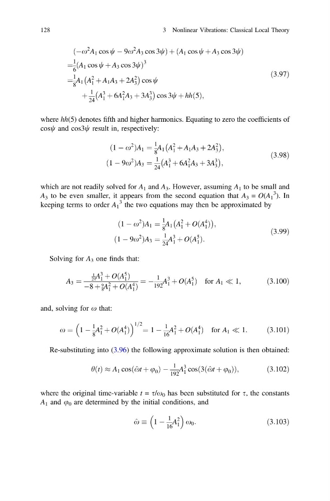
ðÀx
2 A 1 cos w À 9x
2 A 3 cos 3wÞ þ ðA 1 cos w þ A 3 cos 3wÞ
¼
1
6
A 1 cos w þ A 3 cos 3w
ð
Þ
3
¼
1
8
A 1 A
2
1 þ A 1 A 3 þ 2A
2
3
À
Á
cos w
þ
1
24
A
3
1 þ 6A
2
1 A 3 þ 3A
3
3
À
Á
cos 3w þ hhð5Þ;
ð3:97Þ
where hh(5) denotes fifth and higher harmonics. Equating to zero the coefficients of
cosw and cos3w result in, respectively:
ð1 À x
2
ÞA 1 ¼
1
8
A 1 A
2
1 þ A 1 A 3 þ 2A
2
3
À
Á ;
ð1 À 9x
2
ÞA 3 ¼
1
24
A
3
1 þ 6A
2
1 A 3 þ 3A
3
3
À
Á ;
ð3:98Þ
which are not readily solved for A 1 and A 3 . However, assuming A 1 to be small and
A 3 to be even smaller, it appears from the second equation that A 3 = O(A 1
3 ). In
keeping terms to order A 1
3 the two equations may then be approximated by
ð1 À x
2
ÞA 1 ¼
1
8
A 1 A
2
1 þ OðA
4
1 Þ
À
Á ;
ð1 À 9x
2
ÞA 3 ¼
1
24
A
3
1 þ OðA
5
1 Þ:
ð3:99Þ
Solving for A 3 one finds that:
A 3 ¼
1
24 A
3
1 þ OðA
5
1 Þ
À8 þ
9
8 A 2
1 þ OðA 4
1 Þ
¼ À
1
192
A
3
1 þ OðA
5
1 Þ for A 1 ( 1;
ð3:100Þ
and, solving for x that:
x ¼ 1 À
1
8
A
2
1 þ OðA
4
1 Þ
1=2 ¼ 1 À
1
16
A
2
1 þ OðA
4
1 Þ for A 1 ( 1:
ð3:101Þ
Re-substituting into (3.96) the following approximate solution is then obtained:
hðtÞ % A 1 cos ^
xt þ u 0
ð
ÞÀ
1
192
A
3
1 cos 3ð ^
xt þ u 0 Þ
ð
Þ ;
ð3:102Þ
where the original time-variable t = s/x 0 has been substituted for s, the constants
A 1 and u 0 are determined by the initial conditions, and
^
x 1 À
1
16
A
2
1
x 0 :
ð3:103Þ
128
3 Nonlinear Vibrations: Classical Local Theory