

the method, as is its solid basis of mathematical proofs concerning convergence and
accuracy (e.g. Sanders and Verhulst 1985).
An obstacle for the general application of averaging can be to find a transformation of variables that will render a system suitable for averaging, e.g. a system of
the form _
x ¼ efðx; tÞ, x 2 R
n , of which (3.90) for the pendulum is a specific
example. One trick that typically works well is to first find the solution of the
unperturbed system (e = 0) in terms of unknown constants, and then take these
constants as new dependent variables of the perturbed system; this is exactly what is
accomplished by the Van der Pol transformation in (3.85).
We shall return to the method of averaging in Sect. 3.7.4, showing how to use
averaging with forced vibrations.
3.5.6 The Method of Harmonic Balance
With the method of harmonic balance (also called the describing function method)
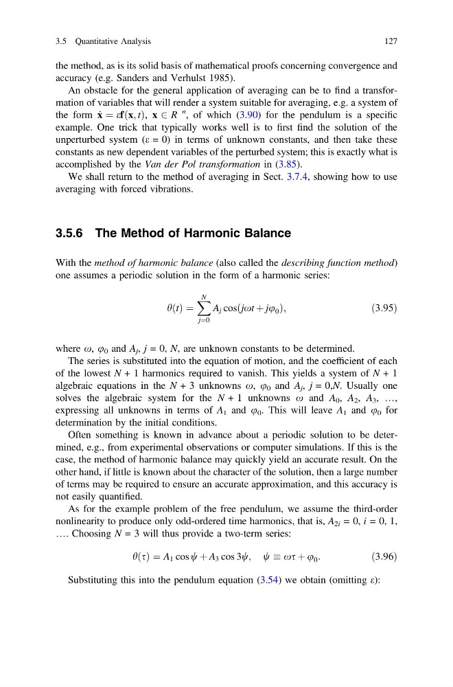
one assumes a periodic solution in the form of a harmonic series:
hðtÞ ¼
X N
j¼0
A j cos jxt þ ju 0
ð
Þ ;
ð3:95Þ
where x, u 0 and A j , j = 0, N, are unknown constants to be determined.
The series is substituted into the equation of motion, and the coefficient of each
of the lowest N + 1 harmonics required to vanish. This yields a system of N + 1
algebraic equations in the N + 3 unknowns x, u 0 and A j , j = 0,N. Usually one
solves the algebraic system for the N + 1 unknowns x and A 0 , A 2 , A 3 , …,
expressing all unknowns in terms of A 1 and u 0 . This will leave A 1 and u 0 for
determination by the initial conditions.
Often something is known in advance about a periodic solution to be determined, e.g., from experimental observations or computer simulations. If this is the
case, the method of harmonic balance may quickly yield an accurate result. On the
other hand, if little is known about the character of the solution, then a large number
of terms may be required to ensure an accurate approximation, and this accuracy is
not easily quantified.
As for the example problem of the free pendulum, we assume the third-order
nonlinearity to produce only odd-ordered time harmonics, that is, A 2i = 0, i = 0, 1,
…. Choosing N = 3 will thus provide a two-term series:
hðsÞ ¼ A 1 cos w þ A 3 cos 3w; w xs þ u 0 :
ð3:96Þ
Substituting this into the pendulum equation (3.54) we obtain (omitting e):
3.5 Quantitative Analysis
127
accuracy (e.g. Sanders and Verhulst 1985).
An obstacle for the general application of averaging can be to find a transformation of variables that will render a system suitable for averaging, e.g. a system of
the form _
x ¼ efðx; tÞ, x 2 R
n , of which (3.90) for the pendulum is a specific
example. One trick that typically works well is to first find the solution of the
unperturbed system (e = 0) in terms of unknown constants, and then take these
constants as new dependent variables of the perturbed system; this is exactly what is
accomplished by the Van der Pol transformation in (3.85).
We shall return to the method of averaging in Sect. 3.7.4, showing how to use
averaging with forced vibrations.
3.5.6 The Method of Harmonic Balance
With the method of harmonic balance (also called the describing function method)
one assumes a periodic solution in the form of a harmonic series:
hðtÞ ¼
X N
j¼0
A j cos jxt þ ju 0
ð
Þ ;
ð3:95Þ
where x, u 0 and A j , j = 0, N, are unknown constants to be determined.
The series is substituted into the equation of motion, and the coefficient of each
of the lowest N + 1 harmonics required to vanish. This yields a system of N + 1
algebraic equations in the N + 3 unknowns x, u 0 and A j , j = 0,N. Usually one
solves the algebraic system for the N + 1 unknowns x and A 0 , A 2 , A 3 , …,
expressing all unknowns in terms of A 1 and u 0 . This will leave A 1 and u 0 for
determination by the initial conditions.
Often something is known in advance about a periodic solution to be determined, e.g., from experimental observations or computer simulations. If this is the
case, the method of harmonic balance may quickly yield an accurate result. On the
other hand, if little is known about the character of the solution, then a large number
of terms may be required to ensure an accurate approximation, and this accuracy is
not easily quantified.
As for the example problem of the free pendulum, we assume the third-order
nonlinearity to produce only odd-ordered time harmonics, that is, A 2i = 0, i = 0, 1,
…. Choosing N = 3 will thus provide a two-term series:
hðsÞ ¼ A 1 cos w þ A 3 cos 3w; w xs þ u 0 :
ð3:96Þ
Substituting this into the pendulum equation (3.54) we obtain (omitting e):
3.5 Quantitative Analysis
127