

Note that a higher harmonic 3 ^
x appears in the response. This too is a nonlinear
feature. It gradually vanishes as the amplitude a 0 ! 0 and the pendulum behaves
increasingly linearly with purely harmonic (i.e. single-frequency sinusoidal)
oscillations. Including more independent time-scales (T 2 , T 3 , …) in the analysis, the
procedure could be continued to yield approximations of even higher order; these
would contain even higher harmonics.
Starting the pendulum from rest with _
h(0) = 0 and h(0) = ~ h 0 , we obtain from
(3.80) that u 0 = 0 and a 0 % ~ h 0 , and hence that:
hðtÞ % ~ h 0 cos ^
xt À
1
192
~ h
3
0 cos 3 ^
xt ; ^
x ¼ 1 À
1
16
~ h
2
o
x 0 :
ð3:82Þ
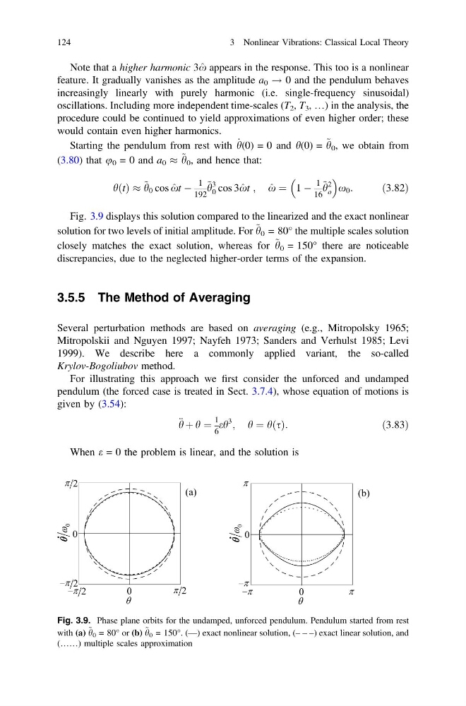
Fig. 3.9 displays this solution compared to the linearized and the exact nonlinear
solution for two levels of initial amplitude. For ~ h 0 = 80° the multiple scales solution
closely matches the exact solution, whereas for ~ h 0 = 150° there are noticeable
discrepancies, due to the neglected higher-order terms of the expansion.
3.5.5 The Method of Averaging
Several perturbation methods are based on averaging (e.g., Mitropolsky 1965;
Mitropolskii and Nguyen 1997; Nayfeh 1973; Sanders and Verhulst 1985; Levi
1999). We describe here a commonly applied variant, the so-called
Krylov-Bogoliubov method.
For illustrating this approach we first consider the unforced and undamped
pendulum (the forced case is treated in Sect. 3.7.4), whose equation of motions is
given by (3.54):
€ h þ h ¼
1
6
eh
3
; h ¼ hðsÞ:
ð3:83Þ
When e = 0 the problem is linear, and the solution is
Fig. 3.9. Phase plane orbits for the undamped, unforced pendulum. Pendulum started from rest
with (a) ~ h 0 = 80° or (b) ~ h 0 = 150°. (—) exact nonlinear solution, (– – –) exact linear solution, and
(……) multiple scales approximation
124
3 Nonlinear Vibrations: Classical Local Theory
x appears in the response. This too is a nonlinear
feature. It gradually vanishes as the amplitude a 0 ! 0 and the pendulum behaves
increasingly linearly with purely harmonic (i.e. single-frequency sinusoidal)
oscillations. Including more independent time-scales (T 2 , T 3 , …) in the analysis, the
procedure could be continued to yield approximations of even higher order; these
would contain even higher harmonics.
Starting the pendulum from rest with _
h(0) = 0 and h(0) = ~ h 0 , we obtain from
(3.80) that u 0 = 0 and a 0 % ~ h 0 , and hence that:
hðtÞ % ~ h 0 cos ^
xt À
1
192
~ h
3
0 cos 3 ^
xt ; ^
x ¼ 1 À
1
16
~ h
2
o
x 0 :
ð3:82Þ
Fig. 3.9 displays this solution compared to the linearized and the exact nonlinear
solution for two levels of initial amplitude. For ~ h 0 = 80° the multiple scales solution
closely matches the exact solution, whereas for ~ h 0 = 150° there are noticeable
discrepancies, due to the neglected higher-order terms of the expansion.
3.5.5 The Method of Averaging
Several perturbation methods are based on averaging (e.g., Mitropolsky 1965;
Mitropolskii and Nguyen 1997; Nayfeh 1973; Sanders and Verhulst 1985; Levi
1999). We describe here a commonly applied variant, the so-called
Krylov-Bogoliubov method.
For illustrating this approach we first consider the unforced and undamped
pendulum (the forced case is treated in Sect. 3.7.4), whose equation of motions is
given by (3.54):
€ h þ h ¼
1
6
eh
3
; h ¼ hðsÞ:
ð3:83Þ
When e = 0 the problem is linear, and the solution is
Fig. 3.9. Phase plane orbits for the undamped, unforced pendulum. Pendulum started from rest
with (a) ~ h 0 = 80° or (b) ~ h 0 = 150°. (—) exact nonlinear solution, (– – –) exact linear solution, and
(……) multiple scales approximation
124
3 Nonlinear Vibrations: Classical Local Theory