

a
0
¼ 0;
1
16
a
3
þ au
0
¼ 0:
ð3:77Þ
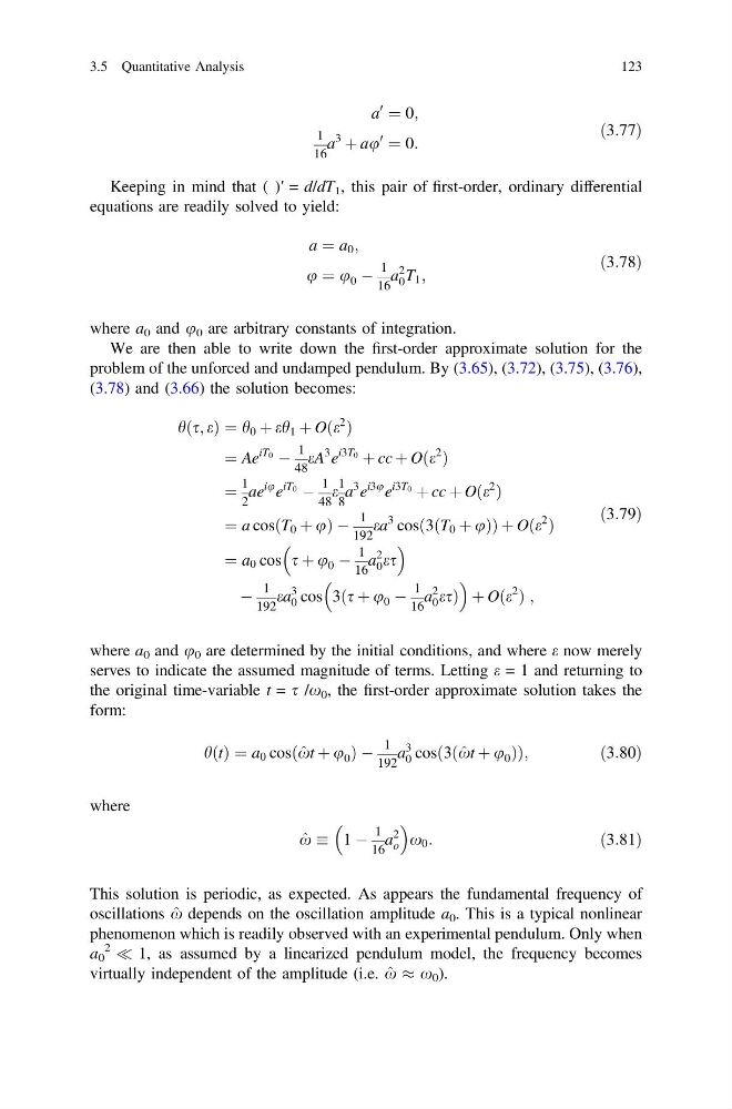
Keeping in mind that ( )′ = d/dT 1 , this pair of first-order, ordinary differential
equations are readily solved to yield:
a ¼ a 0 ;
u ¼ u 0 À
1
16
a
2
0 T 1 ;
ð3:78Þ
where a 0 and u 0 are arbitrary constants of integration.
We are then able to write down the first-order approximate solution for the
problem of the unforced and undamped pendulum. By (3.65), (3.72), (3.75), (3.76),
(3.78) and (3.66) the solution becomes:
hðs; eÞ ¼ h 0 þ eh 1 þ Oðe
2
Þ
¼ Ae
iT 0 À
1
48
eA
3 e
i3T 0 þ cc þ Oðe
2
Þ
¼
1
2
ae
iu e
iT 0 À
1
48
e
1
8
a
3 e
i3u e
i3T 0 þ cc þ Oðe
2
Þ
¼ a cos T 0 þ u
ð
ÞÀ
1
192
ea
3 cos 3ðT 0 þ uÞ
ð
ÞþOðe
2
Þ
¼ a 0 cos s þ u 0 À
1
16
a
2
0 es
À
1
192
ea
3
0 cos 3ðs þ u 0 À
1
16
a
2
0 esÞ
þ Oðe
2
Þ ;
ð3:79Þ
where a 0 and u 0 are determined by the initial conditions, and where e now merely
serves to indicate the assumed magnitude of terms. Letting e = 1 and returning to
the original time-variable t = s /x 0 , the first-order approximate solution takes the
form:
hðtÞ ¼ a 0 cos ^
xt þ u 0
ð
ÞÀ
1
192
a
3
0 cos 3ð ^
xt þ u 0 Þ
ð
Þ ;
ð3:80Þ
where
^
x 1 À
1
16
a
2
o
x 0 :
ð3:81Þ
This solution is periodic, as expected. As appears the fundamental frequency of
oscillations ^
x depends on the oscillation amplitude a 0 . This is a typical nonlinear
phenomenon which is readily observed with an experimental pendulum. Only when
a 0
2
( 1, as assumed by a linearized pendulum model, the frequency becomes
virtually independent of the amplitude (i.e. ^
x % x 0 ).
3.5 Quantitative Analysis
123
0
¼ 0;
1
16
a
3
þ au
0
¼ 0:
ð3:77Þ
Keeping in mind that ( )′ = d/dT 1 , this pair of first-order, ordinary differential
equations are readily solved to yield:
a ¼ a 0 ;
u ¼ u 0 À
1
16
a
2
0 T 1 ;
ð3:78Þ
where a 0 and u 0 are arbitrary constants of integration.
We are then able to write down the first-order approximate solution for the
problem of the unforced and undamped pendulum. By (3.65), (3.72), (3.75), (3.76),
(3.78) and (3.66) the solution becomes:
hðs; eÞ ¼ h 0 þ eh 1 þ Oðe
2
Þ
¼ Ae
iT 0 À
1
48
eA
3 e
i3T 0 þ cc þ Oðe
2
Þ
¼
1
2
ae
iu e
iT 0 À
1
48
e
1
8
a
3 e
i3u e
i3T 0 þ cc þ Oðe
2
Þ
¼ a cos T 0 þ u
ð
ÞÀ
1
192
ea
3 cos 3ðT 0 þ uÞ
ð
ÞþOðe
2
Þ
¼ a 0 cos s þ u 0 À
1
16
a
2
0 es
À
1
192
ea
3
0 cos 3ðs þ u 0 À
1
16
a
2
0 esÞ
þ Oðe
2
Þ ;
ð3:79Þ
where a 0 and u 0 are determined by the initial conditions, and where e now merely
serves to indicate the assumed magnitude of terms. Letting e = 1 and returning to
the original time-variable t = s /x 0 , the first-order approximate solution takes the
form:
hðtÞ ¼ a 0 cos ^
xt þ u 0
ð
ÞÀ
1
192
a
3
0 cos 3ð ^
xt þ u 0 Þ
ð
Þ ;
ð3:80Þ
where
^
x 1 À
1
16
a
2
o
x 0 :
ð3:81Þ
This solution is periodic, as expected. As appears the fundamental frequency of
oscillations ^
x depends on the oscillation amplitude a 0 . This is a typical nonlinear
phenomenon which is readily observed with an experimental pendulum. Only when
a 0
2
( 1, as assumed by a linearized pendulum model, the frequency becomes
virtually independent of the amplitude (i.e. ^
x % x 0 ).
3.5 Quantitative Analysis
123