

(q, X) for which the solution h( t) = 0 becomes unstable and oscillations start
growing. This analysis will predict pendulum rotations h (t) that approach infinity at
exponential rate. As amplitudes grow, however, the linear model becomes
increasingly inadequate, and one needs to drop the assumption sinh % h. Thus,
linear analysis will predict the state h (t) = 0 to be unstable for certain values of
(q,X), while a nonlinear analysis is required for predicting the new (post-critical)
state replacing h (t) = 0.
3.4 Qualitative Analysis of the Unforced Response
3.4.1 Recasting the Equations into First-Order Form
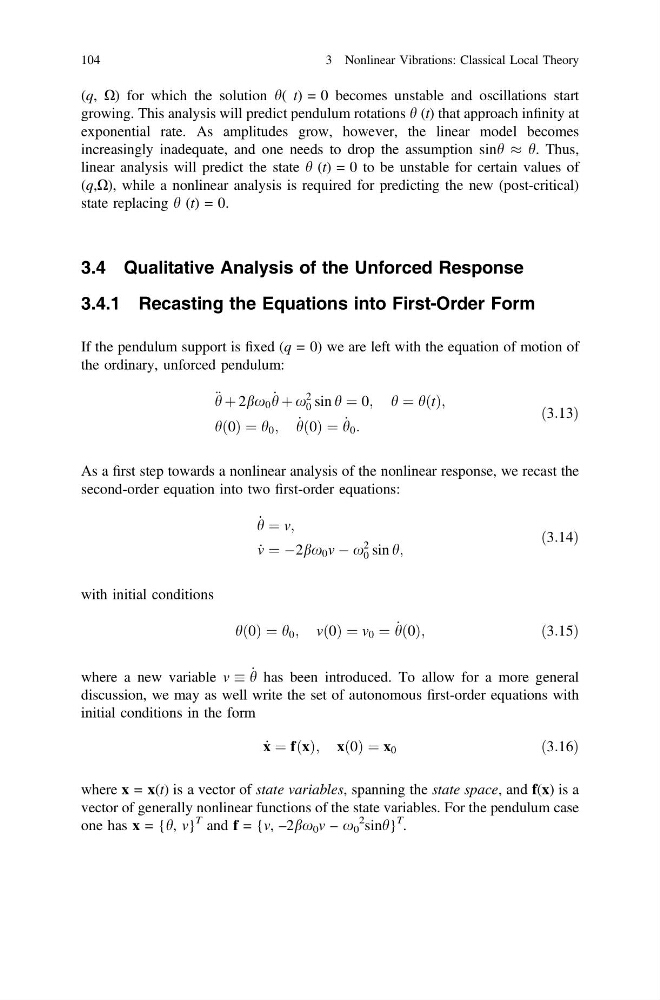
If the pendulum support is fixed (q = 0) we are left with the equation of motion of
the ordinary, unforced pendulum:
€ h þ 2bx 0 _
h þ x
2
0 sin h ¼ 0; h ¼ hðtÞ;
hð0Þ ¼ h 0 ; _
hð0Þ ¼ _
h 0 :
ð3:13Þ
As a first step towards a nonlinear analysis of the nonlinear response, we recast the
second-order equation into two first-order equations:
_
h ¼ v;
_
v ¼ À2bx 0 v À x
2
0 sin h;
ð3:14Þ
with initial conditions
hð0Þ ¼ h 0 ; vð0Þ ¼ v 0 ¼ _
hð0Þ;
ð3:15Þ
where a new variable v _
h has been introduced. To allow for a more general
discussion, we may as well write the set of autonomous first-order equations with
initial conditions in the form
_
x ¼ fðxÞ; xð0Þ ¼ x 0
ð3:16Þ
where x = x(t) is a vector of state variables, spanning the state space, and f(x) is a
vector of generally nonlinear functions of the state variables. For the pendulum case
one has x = {h, v}
T and f = {v, –2bx 0 v – x 0
2 sinh}
T .
104
3 Nonlinear Vibrations: Classical Local Theory
growing. This analysis will predict pendulum rotations h (t) that approach infinity at
exponential rate. As amplitudes grow, however, the linear model becomes
increasingly inadequate, and one needs to drop the assumption sinh % h. Thus,
linear analysis will predict the state h (t) = 0 to be unstable for certain values of
(q,X), while a nonlinear analysis is required for predicting the new (post-critical)
state replacing h (t) = 0.
3.4 Qualitative Analysis of the Unforced Response
3.4.1 Recasting the Equations into First-Order Form
If the pendulum support is fixed (q = 0) we are left with the equation of motion of
the ordinary, unforced pendulum:
€ h þ 2bx 0 _
h þ x
2
0 sin h ¼ 0; h ¼ hðtÞ;
hð0Þ ¼ h 0 ; _
hð0Þ ¼ _
h 0 :
ð3:13Þ
As a first step towards a nonlinear analysis of the nonlinear response, we recast the
second-order equation into two first-order equations:
_
h ¼ v;
_
v ¼ À2bx 0 v À x
2
0 sin h;
ð3:14Þ
with initial conditions
hð0Þ ¼ h 0 ; vð0Þ ¼ v 0 ¼ _
hð0Þ;
ð3:15Þ
where a new variable v _
h has been introduced. To allow for a more general
discussion, we may as well write the set of autonomous first-order equations with
initial conditions in the form
_
x ¼ fðxÞ; xð0Þ ¼ x 0
ð3:16Þ
where x = x(t) is a vector of state variables, spanning the state space, and f(x) is a
vector of generally nonlinear functions of the state variables. For the pendulum case
one has x = {h, v}
T and f = {v, –2bx 0 v – x 0
2 sinh}
T .
104
3 Nonlinear Vibrations: Classical Local Theory