

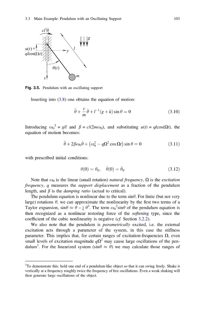
Inserting into (3.8) one obtains the equation of motion:
€ h þ
c
m
_
h þ l
À1 g þ € u
ð
Þsin h ¼ 0
ð3:10Þ
Introducing x 0
2 = g/l and b = c/(2mx 0 ), and substituting u(t) = qlcos(Xt), the
equation of motion becomes:
€ h þ 2bx 0 _
h þ x
2
0 À qX
2 cos Xt
À
Á
sin h ¼ 0
ð3:11Þ
with prescribed initial conditions:
hð0Þ ¼ h 0 ; _
hð0Þ ¼ _
h 0
ð3:12Þ
Note that x 0 is the linear (small rotation) natural frequency, X is the excitation
frequency, q measures the support displacement as a fraction of the pendulum
length, and b is the damping ratio (actual to critical).
The pendulum equation is nonlinear due to the term sinh. For finite (but not very
large) rotations h, we can approximate the nonlinearity by the first two terms of a
Taylor expansion, sinh % h –
1
6 h
3 . The term x 0
2 sinh of the pendulum equation is
then recognized as a nonlinear restoring force of the softening type, since the
coefficient of the cubic nonlinearity is negative (cf. Section 3.2.2).
We also note that the pendulum is parametrically excited, i.e. the external
excitation acts through a parameter of the system, in this case the stiffness
parameter. This implies that, for certain ranges of excitation-frequencies X, even
small levels of excitation magnitude qX
2 may cause large oscillations of the pendulum
1
. For the linearized system (sinh % h) we may calculate those ranges of
Fig. 3.5. Pendulum with an oscillating support
1
To demonstrate this: hold one end of a pendulum-like object so that it can swing freely. Shake it
vertically at a frequency roughly twice the frequency of free oscillations. Even a weak shaking will
then generate large oscillations of the object.
3.3 Main Example: Pendulum with an Oscillating Support
103
€ h þ
c
m
_
h þ l
À1 g þ € u
ð
Þsin h ¼ 0
ð3:10Þ
Introducing x 0
2 = g/l and b = c/(2mx 0 ), and substituting u(t) = qlcos(Xt), the
equation of motion becomes:
€ h þ 2bx 0 _
h þ x
2
0 À qX
2 cos Xt
À
Á
sin h ¼ 0
ð3:11Þ
with prescribed initial conditions:
hð0Þ ¼ h 0 ; _
hð0Þ ¼ _
h 0
ð3:12Þ
Note that x 0 is the linear (small rotation) natural frequency, X is the excitation
frequency, q measures the support displacement as a fraction of the pendulum
length, and b is the damping ratio (actual to critical).
The pendulum equation is nonlinear due to the term sinh. For finite (but not very
large) rotations h, we can approximate the nonlinearity by the first two terms of a
Taylor expansion, sinh % h –
1
6 h
3 . The term x 0
2 sinh of the pendulum equation is
then recognized as a nonlinear restoring force of the softening type, since the
coefficient of the cubic nonlinearity is negative (cf. Section 3.2.2).
We also note that the pendulum is parametrically excited, i.e. the external
excitation acts through a parameter of the system, in this case the stiffness
parameter. This implies that, for certain ranges of excitation-frequencies X, even
small levels of excitation magnitude qX
2 may cause large oscillations of the pendulum
1
. For the linearized system (sinh % h) we may calculate those ranges of
Fig. 3.5. Pendulum with an oscillating support
1
To demonstrate this: hold one end of a pendulum-like object so that it can swing freely. Shake it
vertically at a frequency roughly twice the frequency of free oscillations. Even a weak shaking will
then generate large oscillations of the object.
3.3 Main Example: Pendulum with an Oscillating Support
103