

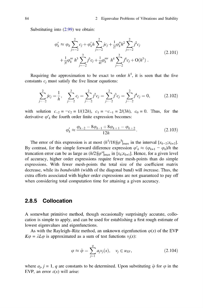
Substituting into (2.99) we obtain:
u
0
k % u k
X 2
j¼À2
c j þ u
0
k h
X 2
j¼À2
jc j þ
1
2!
u
00
k h
2
X 2
j¼À2
j
2 c j
þ
1
3!
u
000
k h
3
X 2
j¼À2
j
3 c j þ
1
4!
u
0000
k h
4
X 2
j¼À2
j
4 c j þ Oðh
5
Þ :
ð2:101Þ
Requiring the approximation to be exact to order h
4 , it is seen that the five
constants c j must satisfy the five linear equations:
X 2
j¼À2
jc j ¼
1
h
;
X 2
j¼À2
c j ¼
X 2
j¼À2
j
2 c j ¼
X 2
j¼À2
j
3 c j ¼
X 2
j¼À2
j
4 c j ¼ 0;
ð2:102Þ
with solution c –2 = −c 2 = 1/(12h), c 1 = −c −1 = 2/(3h), c 0 = 0. Thus, for the
derivative u′ k the fourth order finite expression becomes:
u
0
k %
u kÀ2 À 8u kÀ1 þ 8u k þ 1 À u k þ 2
12h
:
ð2:103Þ
The error of this expression is at most (h
4 /18)|u
5 | max in the interval [x k−2 ;x k+2 ].
By contrast, for the simple forward difference expression u′ k % (u k+1 − u k )/h the
truncation error can be as large as (h/2)|u′′| max in [x k ;x k+1 ]. Hence, for a given level
of accuracy, higher order expressions require fewer mesh-points than do simple
expressions. With fewer mesh-points the total size of the coefficient matrix
decrease, while its bandwidth (width of the diagonal band) will increase. Thus, the
extra efforts associated with higher order expressions are not guaranteed to pay off
when considering total computation time for attaining a given accuracy.
2.8.5 Collocation
A somewhat primitive method, though occasionally surprisingly accurate, collocation is simple to apply, and can be used for establishing a first rough estimate of
lowest eigenvalues and eigenfunctions.
As with the Rayleigh–Ritz method, an unknown eigenfunction u(x) of the EVP
Ku = kLu is approximated as a sum of test functions v j (x):
u % ~
u ¼
X q
j¼1
a j v j ðxÞ; v j 2 u TF ;
ð2:104Þ
where a j , j = 1, q are constants to be determined. Upon substituting ~
u for u in the
EVP, an error e(x) will arise:
84
2 Eigenvalue Problems of Vibrations and Stability
u
0
k % u k
X 2
j¼À2
c j þ u
0
k h
X 2
j¼À2
jc j þ
1
2!
u
00
k h
2
X 2
j¼À2
j
2 c j
þ
1
3!
u
000
k h
3
X 2
j¼À2
j
3 c j þ
1
4!
u
0000
k h
4
X 2
j¼À2
j
4 c j þ Oðh
5
Þ :
ð2:101Þ
Requiring the approximation to be exact to order h
4 , it is seen that the five
constants c j must satisfy the five linear equations:
X 2
j¼À2
jc j ¼
1
h
;
X 2
j¼À2
c j ¼
X 2
j¼À2
j
2 c j ¼
X 2
j¼À2
j
3 c j ¼
X 2
j¼À2
j
4 c j ¼ 0;
ð2:102Þ
with solution c –2 = −c 2 = 1/(12h), c 1 = −c −1 = 2/(3h), c 0 = 0. Thus, for the
derivative u′ k the fourth order finite expression becomes:
u
0
k %
u kÀ2 À 8u kÀ1 þ 8u k þ 1 À u k þ 2
12h
:
ð2:103Þ
The error of this expression is at most (h
4 /18)|u
5 | max in the interval [x k−2 ;x k+2 ].
By contrast, for the simple forward difference expression u′ k % (u k+1 − u k )/h the
truncation error can be as large as (h/2)|u′′| max in [x k ;x k+1 ]. Hence, for a given level
of accuracy, higher order expressions require fewer mesh-points than do simple
expressions. With fewer mesh-points the total size of the coefficient matrix
decrease, while its bandwidth (width of the diagonal band) will increase. Thus, the
extra efforts associated with higher order expressions are not guaranteed to pay off
when considering total computation time for attaining a given accuracy.
2.8.5 Collocation
A somewhat primitive method, though occasionally surprisingly accurate, collocation is simple to apply, and can be used for establishing a first rough estimate of
lowest eigenvalues and eigenfunctions.
As with the Rayleigh–Ritz method, an unknown eigenfunction u(x) of the EVP
Ku = kLu is approximated as a sum of test functions v j (x):
u % ~
u ¼
X q
j¼1
a j v j ðxÞ; v j 2 u TF ;
ð2:104Þ
where a j , j = 1, q are constants to be determined. Upon substituting ~
u for u in the
EVP, an error e(x) will arise:
84
2 Eigenvalue Problems of Vibrations and Stability