

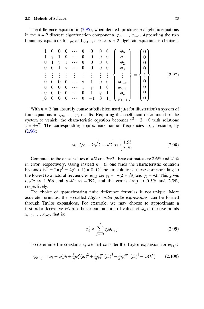
The difference equation in (2.95), when iterated, produces n algebraic equations
in the n + 2 discrete eigenfunction components u 0 , …, u n+1 . Appending the two
boundary equations for u 0 and u n+1 , a set of n + 2 algebraic equations is obtained:
1 0 0 0 Á Á Á 0 0 0 0
1 c 1 0 Á Á Á 0 0 0 0
0 1 c 1 Á Á Á 0 0 0 0
0 0 1 c Á Á Á 0 0 0 0
. .
. . .
. . .
. . .
.
. .
.
. .
.
. .
.
. .
. . .
.
0 0 0 0 Á Á Á c 1 0 0
0 0 0 0 Á Á Á 1 c 1 0
0 0 0 0 Á Á Á 0 1 c 1
0 0 0 0 Á Á Á 0 À1 0 1
2
6
6
6
6
6
6
6
6
6
6
6
6
6
4
3
7
7
7
7
7
7
7
7
7
7
7
7
7
5
u 0
u 1
u 2
u 3
. .
.
u nÀ2
u nÀ1
u n
u n þ 1
8
> > > > > > > > > > > > > <
> > > > > > > > > > > > > :
9
> > > > > > > > > > > > > =
> > > > > > > > > > > > > ;
¼
0
0
0
0
. .
.
0
0
0
0
8
> > > > > > > > > > > > > <
> > > > > > > > > > > > > :
9
> > > > > > > > > > > > > =
> > > > > > > > > > > > > ;
:
ð2:97Þ
With n = 2 (an absurdly coarse subdivision used just for illustration) a system of
four equations in u 0 , …, u 3 results. Requiring the coefficient determinant of the
system to vanish, the characteristic equation becomes c
2
− 2 = 0 with solutions
c = ±√2. The corresponding approximate natural frequencies x 1,2 become, by
(2.96):
x 1;2 l
c ¼ 2
ffiffiffiffiffiffiffiffiffiffiffiffiffiffiffi
2 Æ
ffiffi ffi
2
p
q
%
1:53
3:70
&
ð2:98Þ
Compared to the exact values of p/2 and 3p/2, these estimates are 2.6% and 21%
in error, respectively. Using instead n = 6, one finds the characteristic equation
becomes (c
2
− 2)(c
4
− 4c
2 + 1) = 0. Of the six solutions, those corresponding to
the lowest two natural frequencies x 1,2 are c 1 = –√(2 + √3) and c 2 = √2. This gives
x 1 l/c % 1.566 and x 2 l/c % 4.592, and the errors drop to 0.3% and 2.5%,
respectively.
The choice of approximating finite difference formulas is not unique. More
accurate formulas, the so-called higher order finite expressions, can be formed
through Taylor expansions. For example, we may choose to approximate a
first-order derivative u′ k as a linear combination of values of u k at the five points
x k−2 , …, x k+2 , that is:
u
0
k %
X 2
j¼À2
c j u k þ j :
ð2:99Þ
To determine the constants c j we first consider the Taylor expansion for u k+j :
u k þ j ¼ u k þ u
0
k jh þ
1
2!
u
00
k ðjhÞ
2 þ
1
3!
u
000
k ðjhÞ
3 þ
1
4!
u
0000
k ðjhÞ
4 þ Oðh
5
Þ:
ð2:100Þ
2.8 Methods of Solution
83
in the n + 2 discrete eigenfunction components u 0 , …, u n+1 . Appending the two
boundary equations for u 0 and u n+1 , a set of n + 2 algebraic equations is obtained:
1 0 0 0 Á Á Á 0 0 0 0
1 c 1 0 Á Á Á 0 0 0 0
0 1 c 1 Á Á Á 0 0 0 0
0 0 1 c Á Á Á 0 0 0 0
. .
. . .
. . .
. . .
.
. .
.
. .
.
. .
.
. .
. . .
.
0 0 0 0 Á Á Á c 1 0 0
0 0 0 0 Á Á Á 1 c 1 0
0 0 0 0 Á Á Á 0 1 c 1
0 0 0 0 Á Á Á 0 À1 0 1
2
6
6
6
6
6
6
6
6
6
6
6
6
6
4
3
7
7
7
7
7
7
7
7
7
7
7
7
7
5
u 0
u 1
u 2
u 3
. .
.
u nÀ2
u nÀ1
u n
u n þ 1
8
> > > > > > > > > > > > > <
> > > > > > > > > > > > > :
9
> > > > > > > > > > > > > =
> > > > > > > > > > > > > ;
¼
0
0
0
0
. .
.
0
0
0
0
8
> > > > > > > > > > > > > <
> > > > > > > > > > > > > :
9
> > > > > > > > > > > > > =
> > > > > > > > > > > > > ;
:
ð2:97Þ
With n = 2 (an absurdly coarse subdivision used just for illustration) a system of
four equations in u 0 , …, u 3 results. Requiring the coefficient determinant of the
system to vanish, the characteristic equation becomes c
2
− 2 = 0 with solutions
c = ±√2. The corresponding approximate natural frequencies x 1,2 become, by
(2.96):
x 1;2 l
c ¼ 2
ffiffiffiffiffiffiffiffiffiffiffiffiffiffiffi
2 Æ
ffiffi ffi
2
p
q
%
1:53
3:70
&
ð2:98Þ
Compared to the exact values of p/2 and 3p/2, these estimates are 2.6% and 21%
in error, respectively. Using instead n = 6, one finds the characteristic equation
becomes (c
2
− 2)(c
4
− 4c
2 + 1) = 0. Of the six solutions, those corresponding to
the lowest two natural frequencies x 1,2 are c 1 = –√(2 + √3) and c 2 = √2. This gives
x 1 l/c % 1.566 and x 2 l/c % 4.592, and the errors drop to 0.3% and 2.5%,
respectively.
The choice of approximating finite difference formulas is not unique. More
accurate formulas, the so-called higher order finite expressions, can be formed
through Taylor expansions. For example, we may choose to approximate a
first-order derivative u′ k as a linear combination of values of u k at the five points
x k−2 , …, x k+2 , that is:
u
0
k %
X 2
j¼À2
c j u k þ j :
ð2:99Þ
To determine the constants c j we first consider the Taylor expansion for u k+j :
u k þ j ¼ u k þ u
0
k jh þ
1
2!
u
00
k ðjhÞ
2 þ
1
3!
u
000
k ðjhÞ
3 þ
1
4!
u
0000
k ðjhÞ
4 þ Oðh
5
Þ:
ð2:100Þ
2.8 Methods of Solution
83