

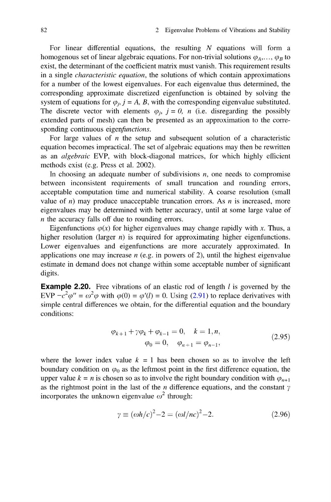
For linear differential equations, the resulting N equations will form a
homogenous set of linear algebraic equations. For non-trivial solutions u A ,…, u B to
exist, the determinant of the coefficient matrix must vanish. This requirement results
in a single characteristic equation, the solutions of which contain approximations
for a number of the lowest eigenvalues. For each eigenvalue thus determined, the
corresponding approximate discretized eigenfunction is obtained by solving the
system of equations for u j , j = A, B, with the corresponding eigenvalue substituted.
The discrete vector with elements u j , j = 0, n (i.e. disregarding the possibly
extended parts of mesh) can then be presented as an approximation to the corresponding continuous eigenfunctions.
For large values of n the setup and subsequent solution of a characteristic
equation becomes impractical. The set of algebraic equations may then be rewritten
as an algebraic EVP, with block-diagonal matrices, for which highly efficient
methods exist (e.g. Press et al. 2002).
In choosing an adequate number of subdivisions n, one needs to compromise
between inconsistent requirements of small truncation and rounding errors,
acceptable computation time and numerical stability. A coarse resolution (small
value of n) may produce unacceptable truncation errors. As n is increased, more
eigenvalues may be determined with better accuracy, until at some large value of
n the accuracy falls off due to rounding errors.
Eigenfunctions u(x) for higher eigenvalues may change rapidly with x. Thus, a
higher resolution (larger n) is required for approximating higher eigenfunctions.
Lower eigenvalues and eigenfunctions are more accurately approximated. In
applications one may increase n (e.g. in powers of 2), until the highest eigenvalue
estimate in demand does not change within some acceptable number of significant
digits.
Example 2.20. Free vibrations of an elastic rod of length l is governed by the
EVP −c
2 u′′ = x
2 u with u(0) = u′(l) = 0. Using (2.91) to replace derivatives with
simple central differences we obtain, for the differential equation and the boundary
conditions:
u k þ 1 þ cu k þ u kÀ1 ¼ 0; k ¼ 1; n;
u 0 ¼ 0; u n þ 1 ¼ u nÀ1 ;
ð2:95Þ
where the lower index value k = 1 has been chosen so as to involve the left
boundary condition on u 0 as the leftmost point in the first difference equation, the
upper value k = n is chosen so as to involve the right boundary condition with u n+1
as the rightmost point in the last of the n difference equations, and the constant c
incorporates the unknown eigenvalue x
2 through:
c xh=c
ð
Þ
2 À2 ¼ xl=nc
ð
Þ
2 À2:
ð2:96Þ
82
2 Eigenvalue Problems of Vibrations and Stability
homogenous set of linear algebraic equations. For non-trivial solutions u A ,…, u B to
exist, the determinant of the coefficient matrix must vanish. This requirement results
in a single characteristic equation, the solutions of which contain approximations
for a number of the lowest eigenvalues. For each eigenvalue thus determined, the
corresponding approximate discretized eigenfunction is obtained by solving the
system of equations for u j , j = A, B, with the corresponding eigenvalue substituted.
The discrete vector with elements u j , j = 0, n (i.e. disregarding the possibly
extended parts of mesh) can then be presented as an approximation to the corresponding continuous eigenfunctions.
For large values of n the setup and subsequent solution of a characteristic
equation becomes impractical. The set of algebraic equations may then be rewritten
as an algebraic EVP, with block-diagonal matrices, for which highly efficient
methods exist (e.g. Press et al. 2002).
In choosing an adequate number of subdivisions n, one needs to compromise
between inconsistent requirements of small truncation and rounding errors,
acceptable computation time and numerical stability. A coarse resolution (small
value of n) may produce unacceptable truncation errors. As n is increased, more
eigenvalues may be determined with better accuracy, until at some large value of
n the accuracy falls off due to rounding errors.
Eigenfunctions u(x) for higher eigenvalues may change rapidly with x. Thus, a
higher resolution (larger n) is required for approximating higher eigenfunctions.
Lower eigenvalues and eigenfunctions are more accurately approximated. In
applications one may increase n (e.g. in powers of 2), until the highest eigenvalue
estimate in demand does not change within some acceptable number of significant
digits.
Example 2.20. Free vibrations of an elastic rod of length l is governed by the
EVP −c
2 u′′ = x
2 u with u(0) = u′(l) = 0. Using (2.91) to replace derivatives with
simple central differences we obtain, for the differential equation and the boundary
conditions:
u k þ 1 þ cu k þ u kÀ1 ¼ 0; k ¼ 1; n;
u 0 ¼ 0; u n þ 1 ¼ u nÀ1 ;
ð2:95Þ
where the lower index value k = 1 has been chosen so as to involve the left
boundary condition on u 0 as the leftmost point in the first difference equation, the
upper value k = n is chosen so as to involve the right boundary condition with u n+1
as the rightmost point in the last of the n difference equations, and the constant c
incorporates the unknown eigenvalue x
2 through:
c xh=c
ð
Þ
2 À2 ¼ xl=nc
ð
Þ
2 À2:
ð2:96Þ
82
2 Eigenvalue Problems of Vibrations and Stability