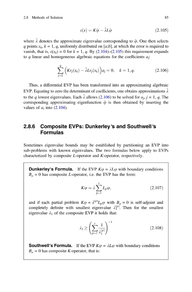
eðxÞ ¼ K ~
u À ~ kL~ u
ð2:105Þ
where ~ k denotes the approximate eigenvalue corresponding to ~
u. One then selects
q points x k , k = 1, q, uniformly distributed on [a;b], at which the error is required to
vanish, that is, e(x k ) = 0 for k = 1, q. By (2.104)–(2.105) this requirement expands
to q linear and homogeneous algebraic equations for the coefficients a j :
X q
j¼1
Kv j ðx k Þ À ~ kLv j ðx k Þ
a j ¼ 0; k ¼ 1; q:
ð2:106Þ
Thus, a differential EVP has been transformed into an approximating algebraic
EVP. Equating to zero the determinant of coefficients, one obtains approximations ~ k
to the q lowest eigenvalues. Each ~ k allows (2.106) to be solved for a j , j = 1, q. The
corresponding approximating eigenfunction ~
u is then obtained by inserting the
values of a i into (2.104).
2.8.6 Composite EVPs: Dunkerley’s and Southwell’s
Formulas
Sometimes eigenvalue bounds may be established by partitioning an EVP into
sub-problems with known eigenvalues. The two formulas below apply to EVPs
characterized by composite L-operator and K-operator, respectively.
Dunkerley’s Formula. If the EVP Ku = kLu with boundary conditions
B l = 0 has composite L-operator, i.e. the EVP has the form:
Ku ¼ k
X r
p¼1
L p u;
ð2:107Þ
and if each partial problem Ku = k
(p) L p u with B l = 0 is self-adjoint and
completely definite with smallest eigenvalue k 1
(p)
. Then for the smallest
eigenvalue k 1 of the composite EVP it holds that:
k 1 !
X r
p¼1
1
k
ðpÞ
1
! À1
ð2:108Þ
Southwell’s Formula. If the EVP Ku = kLu with boundary conditions
B l = 0 has composite K-operator, that is:
2.8 Methods of Solution
85