

5.6 Geometrically Nonlinear FE Models
91
1 M uu
2
0 ¨
q +
1 K uu q +
1 K uφ φ a = F ue −
1 F ui ,
(5.67)
1 K φu q +
1 K φφ φ s = G φe −
1 G φi ,
(5.68)
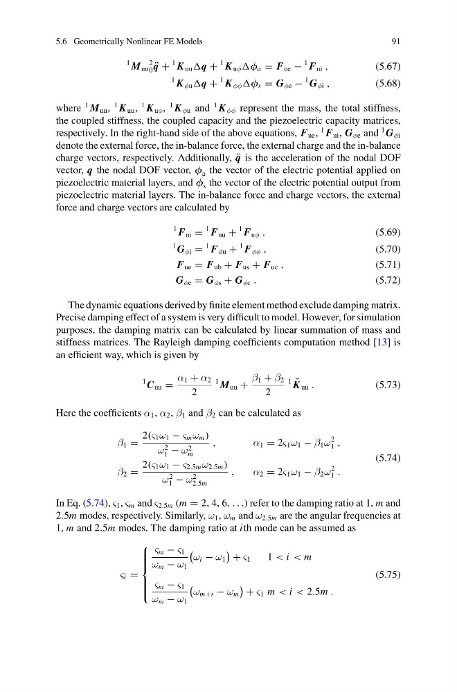
where
1 M uu ,
1 K uu ,
1 K uφ ,
1 K φu and
1 K φφ represent the mass, the total stiffness,
the coupled stiffness, the coupled capacity and the piezoelectric capacity matrices,
respectively. In the right-hand side of the above equations, F ue ,
1 F ui , G φe and
1 G φi
denote the external force, the in-balance force, the external charge and the in-balance
charge vectors, respectively. Additionally, ¨
q is the acceleration of the nodal DOF
vector, q the nodal DOF vector, φ a the vector of the electric potential applied on
piezoelectric material layers, and φ s the vector of the electric potential output from
piezoelectric material layers. The in-balance force and charge vectors, the external
force and charge vectors are calculated by
1 F ui =
1 F uu +
1 F uφ ,
(5.69)
1 G φi =
1 F φu +
1 F φφ ,
(5.70)
F ue = F ub + F us + F uc ,
(5.71)
G φe = G φs + G φc .
(5.72)
The dynamic equations derived by finite element method exclude damping matrix.
Precise damping effect of a system is very difficult to model. However, for simulation
purposes, the damping matrix can be calculated by linear summation of mass and
stiffness matrices. The Rayleigh damping coefficients computation method [13] is
an efficient way, which is given by
1 C uu =
α 1 + α 2
2
1 M uu +
β 1 + β 2
2
1 ¯
K uu .
(5.73)
Here the coefficients α 1 , α 2 , β 1 and β 2 can be calculated as
β 1 =
2(ς 1 ω 1 − ς m ω m )
ω
2
1 − ω 2
m
,
α 1 = 2ς 1 ω 1 − β 1 ω
2
1 ,
β 2 =
2(ς 1 ω 1 − ς 2.5m ω 2.5m )
ω
2
1 − ω
2
2.5m
,
α 2 = 2ς 1 ω 1 − β 2 ω
2
1 .
(5.74)
In Eq. (5.74), ς 1 , ς m and ς 2.5m (m = 2, 4, 6, . . .) refer to the damping ratio at 1, m and
2.5m modes, respectively. Similarly, ω 1 , ω m and ω 2.5m are the angular frequencies at
1, m and 2.5m modes. The damping ratio at ith mode can be assumed as
ς i =
⎧
⎪ ⎪ ⎪ ⎨
⎪ ⎪ ⎪ ⎩
ς m − ς 1
ω m − ω 1
ω i − ω 1
+ ς 1
1 < i < m
ς m − ς 1
ω m − ω 1
ω m+i − ω m
+ ς 1 m < i < 2.5m .
(5.75)
91
1 M uu
2
0 ¨
q +
1 K uu q +
1 K uφ φ a = F ue −
1 F ui ,
(5.67)
1 K φu q +
1 K φφ φ s = G φe −
1 G φi ,
(5.68)
where
1 M uu ,
1 K uu ,
1 K uφ ,
1 K φu and
1 K φφ represent the mass, the total stiffness,
the coupled stiffness, the coupled capacity and the piezoelectric capacity matrices,
respectively. In the right-hand side of the above equations, F ue ,
1 F ui , G φe and
1 G φi
denote the external force, the in-balance force, the external charge and the in-balance
charge vectors, respectively. Additionally, ¨
q is the acceleration of the nodal DOF
vector, q the nodal DOF vector, φ a the vector of the electric potential applied on
piezoelectric material layers, and φ s the vector of the electric potential output from
piezoelectric material layers. The in-balance force and charge vectors, the external
force and charge vectors are calculated by
1 F ui =
1 F uu +
1 F uφ ,
(5.69)
1 G φi =
1 F φu +
1 F φφ ,
(5.70)
F ue = F ub + F us + F uc ,
(5.71)
G φe = G φs + G φc .
(5.72)
The dynamic equations derived by finite element method exclude damping matrix.
Precise damping effect of a system is very difficult to model. However, for simulation
purposes, the damping matrix can be calculated by linear summation of mass and
stiffness matrices. The Rayleigh damping coefficients computation method [13] is
an efficient way, which is given by
1 C uu =
α 1 + α 2
2
1 M uu +
β 1 + β 2
2
1 ¯
K uu .
(5.73)
Here the coefficients α 1 , α 2 , β 1 and β 2 can be calculated as
β 1 =
2(ς 1 ω 1 − ς m ω m )
ω
2
1 − ω 2
m
,
α 1 = 2ς 1 ω 1 − β 1 ω
2
1 ,
β 2 =
2(ς 1 ω 1 − ς 2.5m ω 2.5m )
ω
2
1 − ω
2
2.5m
,
α 2 = 2ς 1 ω 1 − β 2 ω
2
1 .
(5.74)
In Eq. (5.74), ς 1 , ς m and ς 2.5m (m = 2, 4, 6, . . .) refer to the damping ratio at 1, m and
2.5m modes, respectively. Similarly, ω 1 , ω m and ω 2.5m are the angular frequencies at
1, m and 2.5m modes. The damping ratio at ith mode can be assumed as
ς i =
⎧
⎪ ⎪ ⎪ ⎨
⎪ ⎪ ⎪ ⎩
ς m − ς 1
ω m − ω 1
ω i − ω 1
+ ς 1
1 < i < m
ς m − ς 1
ω m − ω 1
ω m+i − ω m
+ ς 1 m < i < 2.5m .
(5.75)