

244
5 Contraction
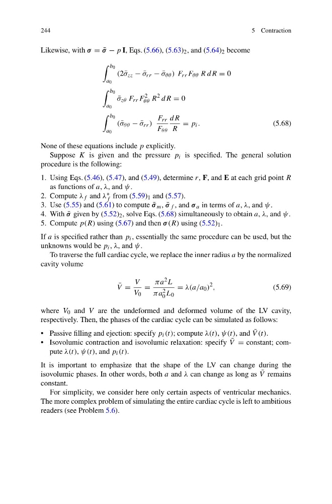
Likewise, with σ = ¯
σ − p I, Eqs. (5.66), (5.63) 2 , and (5.64) 2 become
b 0
a 0
(2 ¯
σ zz − ¯
σ rr − ¯
σ θθ ) F rr F θθ R dR = 0
b 0
a 0
¯
σ zθ F rr F
2
θθ R
2 dR = 0
b 0
a 0
( ¯
σ θθ − ¯
σ rr )
F rr
F θθ
dR
R
= p i .
(5.68)
None of these equations include p explicitly.
Suppose K is given and the pressure p i is specified. The general solution
procedure is the following:
1. Using Eqs. (5.46), (5.47), and (5.49), determine r, F, and E at each grid point R
as functions of a, λ, and ψ.
2. Compute λ f and λ ∗
f from (5.59) 1 and (5.57).
3. Use (5.55) and (5.61) to compute ¯
σ m , ¯
σ f , and σ a in terms of a, λ, and ψ.
4. With ¯
σ given by (5.52) 2 , solve Eqs. (5.68) simultaneously to obtain a, λ, and ψ.
5. Compute p(R) using (5.67) and then σ (R) using (5.52) 1 .
If a is specified rather than p i , essentially the same procedure can be used, but the
unknowns would be p i , λ, and ψ.
To traverse the full cardiac cycle, we replace the inner radius a by the normalized
cavity volume
¯
V =
V
V 0
=
πa 2 L
πa 2
0 L 0
= λ(a/a 0 )
2 ,
(5.69)
where V 0 and V are the undeformed and deformed volume of the LV cavity,
respectively. Then, the phases of the cardiac cycle can be simulated as follows:
• Passive filling and ejection: specify p i (t); compute λ(t), ψ(t), and ¯
V (t).
• Isovolumic contraction and isovolumic relaxation: specify ¯
V = constant; compute λ(t), ψ(t), and p i (t).
It is important to emphasize that the shape of the LV can change during the
isovolumic phases. In other words, both a and λ can change as long as ¯
V remains
constant.
For simplicity, we consider here only certain aspects of ventricular mechanics.
The more complex problem of simulating the entire cardiac cycle is left to ambitious
readers (see Problem 5.6).
5 Contraction
Likewise, with σ = ¯
σ − p I, Eqs. (5.66), (5.63) 2 , and (5.64) 2 become
b 0
a 0
(2 ¯
σ zz − ¯
σ rr − ¯
σ θθ ) F rr F θθ R dR = 0
b 0
a 0
¯
σ zθ F rr F
2
θθ R
2 dR = 0
b 0
a 0
( ¯
σ θθ − ¯
σ rr )
F rr
F θθ
dR
R
= p i .
(5.68)
None of these equations include p explicitly.
Suppose K is given and the pressure p i is specified. The general solution
procedure is the following:
1. Using Eqs. (5.46), (5.47), and (5.49), determine r, F, and E at each grid point R
as functions of a, λ, and ψ.
2. Compute λ f and λ ∗
f from (5.59) 1 and (5.57).
3. Use (5.55) and (5.61) to compute ¯
σ m , ¯
σ f , and σ a in terms of a, λ, and ψ.
4. With ¯
σ given by (5.52) 2 , solve Eqs. (5.68) simultaneously to obtain a, λ, and ψ.
5. Compute p(R) using (5.67) and then σ (R) using (5.52) 1 .
If a is specified rather than p i , essentially the same procedure can be used, but the
unknowns would be p i , λ, and ψ.
To traverse the full cardiac cycle, we replace the inner radius a by the normalized
cavity volume
¯
V =
V
V 0
=
πa 2 L
πa 2
0 L 0
= λ(a/a 0 )
2 ,
(5.69)
where V 0 and V are the undeformed and deformed volume of the LV cavity,
respectively. Then, the phases of the cardiac cycle can be simulated as follows:
• Passive filling and ejection: specify p i (t); compute λ(t), ψ(t), and ¯
V (t).
• Isovolumic contraction and isovolumic relaxation: specify ¯
V = constant; compute λ(t), ψ(t), and p i (t).
It is important to emphasize that the shape of the LV can change during the
isovolumic phases. In other words, both a and λ can change as long as ¯
V remains
constant.
For simplicity, we consider here only certain aspects of ventricular mechanics.
The more complex problem of simulating the entire cardiac cycle is left to ambitious
readers (see Problem 5.6).