

5.5 Case Study: Cardiac Mechanics
245
5.5.6 Illustrative Results
Unless indicated otherwise, all results are based on the following representative
parameter values for the canine LV:
a 0 = 1.4 cm
b 0 = 2.6 cm
β 0 = 60 ◦
φ p = 0.2
φ a = 0.8
c m = 2.5 kPa
α m = 2
c f = 1.5 kPa
α f = 1
c a , max = 3 kPa K min = 0.7
.
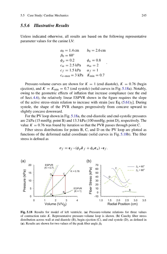
Pressure-volume curves are shown for K = 1 (end diastole), K = 0.76 (begin
ejection), and K = K min = 0.7 (end systole) (solid curves in Fig. 5.18a). Notably,
owing to the geometric effects of inflation that increase compliance (see the end
of Sect. 4.6), the relatively linear ESPVR shown in the figure requires the slope
of the active stress-strain relation to increase with strain [see Eq. (5.61) 2 ]. During
systole, the shape of the PVR changes progressively from concave upward to
slightly concave downward.
For the PV loop shown in Fig. 5.18a, the end-diastolic and end-systolic pressures
are 2 kPa (15 mmHg; point B) and 13.3 kPa (100 mmHg; point D), respectively. The
value K = 0.76 was found by iteration so that the PVR passes through point C.
Fiber stress distributions for points B, C, and D on the PV loop are plotted as
functions of the deformed radial coordinate (solid curves in Fig. 5.18b). The fiber
stress is defined as
σ f = e f · (φ p ¯
σ f + φ a σ a ) · e f .
Fig. 5.18 Results for model of left ventricle. (a) Pressure-volume relations for three values
of contraction ratio K. Representative pressure-volume loop is shown. (b) Cauchy fiber stress
distribution across wall at end diastole (B), begin ejection (C), and end systole (D), as defined in
(a). Results are shown for two values of the peak fiber angle β 0
245
5.5.6 Illustrative Results
Unless indicated otherwise, all results are based on the following representative
parameter values for the canine LV:
a 0 = 1.4 cm
b 0 = 2.6 cm
β 0 = 60 ◦
φ p = 0.2
φ a = 0.8
c m = 2.5 kPa
α m = 2
c f = 1.5 kPa
α f = 1
c a , max = 3 kPa K min = 0.7
.
Pressure-volume curves are shown for K = 1 (end diastole), K = 0.76 (begin
ejection), and K = K min = 0.7 (end systole) (solid curves in Fig. 5.18a). Notably,
owing to the geometric effects of inflation that increase compliance (see the end
of Sect. 4.6), the relatively linear ESPVR shown in the figure requires the slope
of the active stress-strain relation to increase with strain [see Eq. (5.61) 2 ]. During
systole, the shape of the PVR changes progressively from concave upward to
slightly concave downward.
For the PV loop shown in Fig. 5.18a, the end-diastolic and end-systolic pressures
are 2 kPa (15 mmHg; point B) and 13.3 kPa (100 mmHg; point D), respectively. The
value K = 0.76 was found by iteration so that the PVR passes through point C.
Fiber stress distributions for points B, C, and D on the PV loop are plotted as
functions of the deformed radial coordinate (solid curves in Fig. 5.18b). The fiber
stress is defined as
σ f = e f · (φ p ¯
σ f + φ a σ a ) · e f .
Fig. 5.18 Results for model of left ventricle. (a) Pressure-volume relations for three values
of contraction ratio K. Representative pressure-volume loop is shown. (b) Cauchy fiber stress
distribution across wall at end diastole (B), begin ejection (C), and end systole (D), as defined in
(a). Results are shown for two values of the peak fiber angle β 0