

4.7 Bending of a Block
199
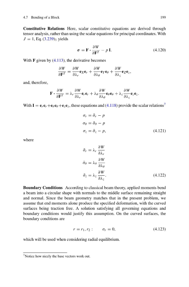
Constitutive Relations Here, scalar constitutive equations are derived through
tensor analysis, rather than using the scalar equations for principal coordinates. With
J = 1, Eq. (3.239) 1 yields
σ = F ·
∂W
∂F T − p I.
(4.120)
With F given by (4.113), the derivative becomes
∂W
∂F T =
∂W
∂λ r
e X e r +
∂W
∂λ θ
e Y e θ +
∂W
∂λ z
e Z e z ,
and, therefore,
F ·
∂W
∂F T = λ r
∂W
∂λ r
e r e r + λ θ
∂W
∂λ θ
e θ e θ + λ z
∂W
∂λ z
e z e z .
With I = e r e r +e θ e θ +e z e z , these equations and (4.118) provide the scalar relations 7
σ r = ¯
σ r − p
σ θ = ¯
σ θ − p
σ z = ¯
σ z − p,
(4.121)
where
¯
σ r = λ r
∂W
∂λ r
¯
σ θ = λ θ
∂W
∂λ θ
¯
σ z = λ z
∂W
∂λ z
.
(4.122)
Boundary Conditions According to classical beam theory, applied moments bend
a beam into a circular shape with normals to the middle surface remaining straight
and normal. Since the beam geometry matches that in the present problem, we
assume that end moments alone produce the specified deformation, with the curved
surfaces being traction free. A solution satisfying all governing equations and
boundary conditions would justify this assumption. On the curved surfaces, the
boundary conditions are
r = r 1 , r 2 :
σ r = 0,
(4.123)
which will be used when considering radial equilibrium.
7 Notice how nicely the base vectors work out.
199
Constitutive Relations Here, scalar constitutive equations are derived through
tensor analysis, rather than using the scalar equations for principal coordinates. With
J = 1, Eq. (3.239) 1 yields
σ = F ·
∂W
∂F T − p I.
(4.120)
With F given by (4.113), the derivative becomes
∂W
∂F T =
∂W
∂λ r
e X e r +
∂W
∂λ θ
e Y e θ +
∂W
∂λ z
e Z e z ,
and, therefore,
F ·
∂W
∂F T = λ r
∂W
∂λ r
e r e r + λ θ
∂W
∂λ θ
e θ e θ + λ z
∂W
∂λ z
e z e z .
With I = e r e r +e θ e θ +e z e z , these equations and (4.118) provide the scalar relations 7
σ r = ¯
σ r − p
σ θ = ¯
σ θ − p
σ z = ¯
σ z − p,
(4.121)
where
¯
σ r = λ r
∂W
∂λ r
¯
σ θ = λ θ
∂W
∂λ θ
¯
σ z = λ z
∂W
∂λ z
.
(4.122)
Boundary Conditions According to classical beam theory, applied moments bend
a beam into a circular shape with normals to the middle surface remaining straight
and normal. Since the beam geometry matches that in the present problem, we
assume that end moments alone produce the specified deformation, with the curved
surfaces being traction free. A solution satisfying all governing equations and
boundary conditions would justify this assumption. On the curved surfaces, the
boundary conditions are
r = r 1 , r 2 :
σ r = 0,
(4.123)
which will be used when considering radial equilibrium.
7 Notice how nicely the base vectors work out.