

4.3 Shear of a Block
173
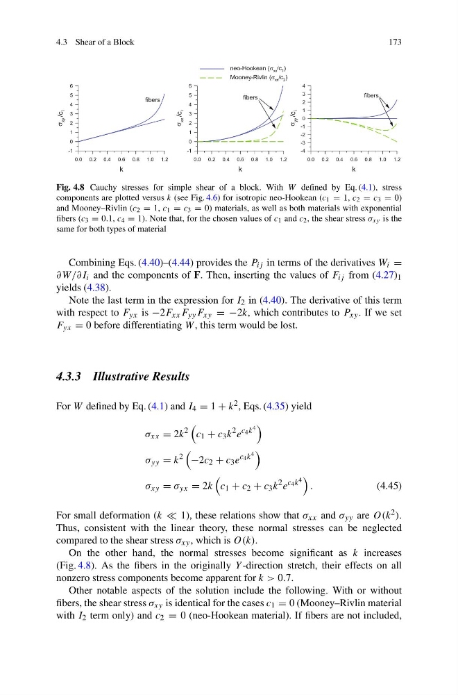
Fig. 4.8 Cauchy stresses for simple shear of a block. With W defined by Eq. (4.1), stress
components are plotted versus k (see Fig. 4.6) for isotropic neo-Hookean (c 1 = 1, c 2 = c 3 = 0)
and Mooney–Rivlin (c 2 = 1, c 1 = c 3 = 0) materials, as well as both materials with exponential
fibers (c 3 = 0.1, c 4 = 1). Note that, for the chosen values of c 1 and c 2 , the shear stress σ xy is the
same for both types of material
Combining Eqs. (4.40)–(4.44) provides the P ij in terms of the derivatives W i =
∂W/∂I i and the components of F. Then, inserting the values of F ij from (4.27) 1
yields (4.38).
Note the last term in the expression for I 2 in (4.40). The derivative of this term
with respect to F yx is −2F xx F yy F xy = −2k, which contributes to P xy . If we set
F yx = 0 before differentiating W , this term would be lost.
4.3.3 Illustrative Results
For W defined by Eq. (4.1) and I 4 = 1 + k 2 , Eqs. (4.35) yield
σ xx = 2k
2
c 1 + c 3 k
2 e
c 4 k 4
σ yy = k
2
−2c 2 + c 3 e
c 4 k 4
σ xy = σ yx = 2k
c 1 + c 2 + c 3 k
2 e
c 4 k 4
.
(4.45)
For small deformation (k 1), these relations show that σ xx and σ yy are O(k 2 ).
Thus, consistent with the linear theory, these normal stresses can be neglected
compared to the shear stress σ xy , which is O(k).
On the other hand, the normal stresses become significant as k increases
(Fig. 4.8). As the fibers in the originally Y -direction stretch, their effects on all
nonzero stress components become apparent for k > 0.7.
Other notable aspects of the solution include the following. With or without
fibers, the shear stress σ xy is identical for the cases c 1 = 0 (Mooney–Rivlin material
with I 2 term only) and c 2 = 0 (neo-Hookean material). If fibers are not included,
173
Fig. 4.8 Cauchy stresses for simple shear of a block. With W defined by Eq. (4.1), stress
components are plotted versus k (see Fig. 4.6) for isotropic neo-Hookean (c 1 = 1, c 2 = c 3 = 0)
and Mooney–Rivlin (c 2 = 1, c 1 = c 3 = 0) materials, as well as both materials with exponential
fibers (c 3 = 0.1, c 4 = 1). Note that, for the chosen values of c 1 and c 2 , the shear stress σ xy is the
same for both types of material
Combining Eqs. (4.40)–(4.44) provides the P ij in terms of the derivatives W i =
∂W/∂I i and the components of F. Then, inserting the values of F ij from (4.27) 1
yields (4.38).
Note the last term in the expression for I 2 in (4.40). The derivative of this term
with respect to F yx is −2F xx F yy F xy = −2k, which contributes to P xy . If we set
F yx = 0 before differentiating W , this term would be lost.
4.3.3 Illustrative Results
For W defined by Eq. (4.1) and I 4 = 1 + k 2 , Eqs. (4.35) yield
σ xx = 2k
2
c 1 + c 3 k
2 e
c 4 k 4
σ yy = k
2
−2c 2 + c 3 e
c 4 k 4
σ xy = σ yx = 2k
c 1 + c 2 + c 3 k
2 e
c 4 k 4
.
(4.45)
For small deformation (k 1), these relations show that σ xx and σ yy are O(k 2 ).
Thus, consistent with the linear theory, these normal stresses can be neglected
compared to the shear stress σ xy , which is O(k).
On the other hand, the normal stresses become significant as k increases
(Fig. 4.8). As the fibers in the originally Y -direction stretch, their effects on all
nonzero stress components become apparent for k > 0.7.
Other notable aspects of the solution include the following. With or without
fibers, the shear stress σ xy is identical for the cases c 1 = 0 (Mooney–Rivlin material
with I 2 term only) and c 2 = 0 (neo-Hookean material). If fibers are not included,