

172
4 Problems in Soft Tissue Biomechanics
F =
⎡
⎣
F xx F xy 0
F yx F yy 0
0 0 F zz
⎤
⎦ ,
(4.39)
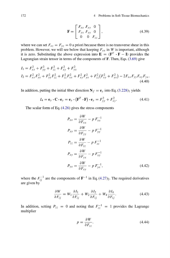
where we can set F xz = F yz = 0 a priori because there is no transverse shear in this
problem. However, we will see below that keeping F yx in W is important, although
it is zero. Substituting the above expression into E = (F T · F − I) provides the
Lagrangian strain tensor in terms of the components of F. Then, Eqs. (3.69) give
I 1 = F
2
xx + F
2
yy + F
2
zz + F
2
xy + F
2
yx
I 2 = F
2
xx F
2
yy + F
2
yy F
2
zz + F
2
zz F
2
xx + F
2
xy F
2
yx + F
2
zz
F
2
xy + F
2
yx
− 2F xx F yy F xy F yx .
(4.40)
In addition, putting the initial fiber direction N f = e y into Eq. (3.228) 1 yields
I 4 = e y · C · e y = e y ·
F
T
· F
· e y = F
2
yy + F
2
xy .
(4.41)
The scalar form of Eq. (4.26) gives the stress components
P xx =
∂W
∂F xx
− p F
−1
xx
P yy =
∂W
∂F yy
− p F
−1
yy
P zz =
∂W
∂F zz
− p F
−1
zz
P xy =
∂W
∂F yx
− p F
−1
xy
P yx =
∂W
∂F xy
− p F
−1
yx ,
(4.42)
where the F
−1
ij are the components of F −1 in Eq. (4.27) 2 . The required derivatives
are given by
∂W
∂F ij
= W 1
∂I 1
∂F ij
+ W 2
∂I 2
∂F ij
+ W 4
∂I 4
∂F ij
.
(4.43)
In addition, setting P zz = 0 and noting that F −1
zz = 1 provides the Lagrange
multiplier
p =
∂W
∂F zz
.
(4.44)
4 Problems in Soft Tissue Biomechanics
F =
⎡
⎣
F xx F xy 0
F yx F yy 0
0 0 F zz
⎤
⎦ ,
(4.39)
where we can set F xz = F yz = 0 a priori because there is no transverse shear in this
problem. However, we will see below that keeping F yx in W is important, although
it is zero. Substituting the above expression into E = (F T · F − I) provides the
Lagrangian strain tensor in terms of the components of F. Then, Eqs. (3.69) give
I 1 = F
2
xx + F
2
yy + F
2
zz + F
2
xy + F
2
yx
I 2 = F
2
xx F
2
yy + F
2
yy F
2
zz + F
2
zz F
2
xx + F
2
xy F
2
yx + F
2
zz
F
2
xy + F
2
yx
− 2F xx F yy F xy F yx .
(4.40)
In addition, putting the initial fiber direction N f = e y into Eq. (3.228) 1 yields
I 4 = e y · C · e y = e y ·
F
T
· F
· e y = F
2
yy + F
2
xy .
(4.41)
The scalar form of Eq. (4.26) gives the stress components
P xx =
∂W
∂F xx
− p F
−1
xx
P yy =
∂W
∂F yy
− p F
−1
yy
P zz =
∂W
∂F zz
− p F
−1
zz
P xy =
∂W
∂F yx
− p F
−1
xy
P yx =
∂W
∂F xy
− p F
−1
yx ,
(4.42)
where the F
−1
ij are the components of F −1 in Eq. (4.27) 2 . The required derivatives
are given by
∂W
∂F ij
= W 1
∂I 1
∂F ij
+ W 2
∂I 2
∂F ij
+ W 4
∂I 4
∂F ij
.
(4.43)
In addition, setting P zz = 0 and noting that F −1
zz = 1 provides the Lagrange
multiplier
p =
∂W
∂F zz
.
(4.44)