

52
P. Liu
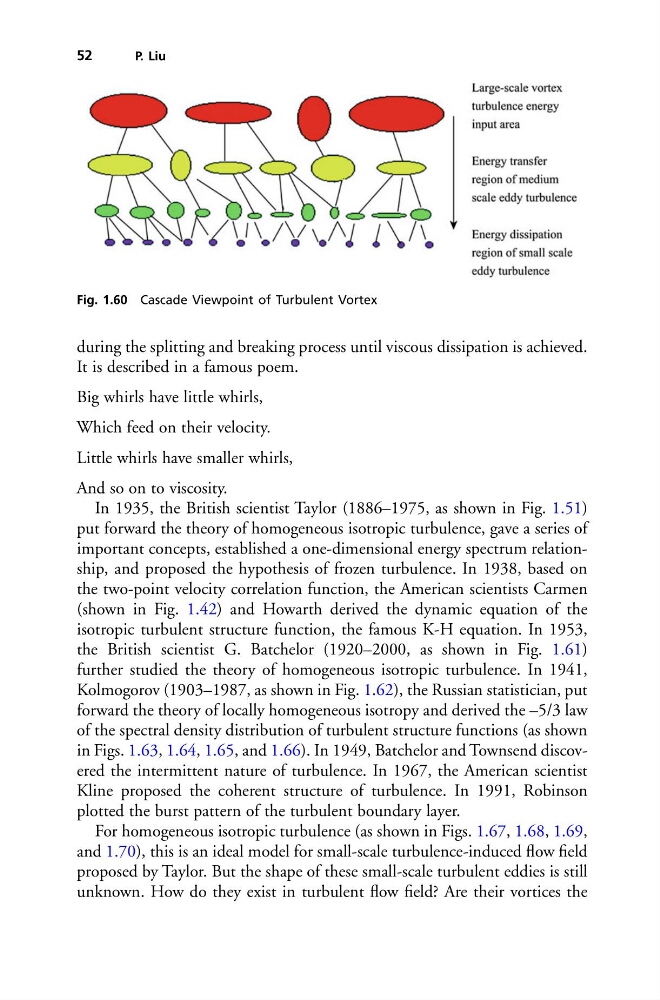
Fig. 1.60 Cascade Viewpoint of Turbulent Vortex
during the splitting and breaking process until viscous dissipation is achieved.
It is described in a famous poem.
Big whirls have little whirls,
Which feed on their velocity.
Little whirls have smaller whirls,
And so on to viscosity.
In 1935, the British scientist Taylor (1886–1975, as shown in Fig. 1.51)
put forward the theory of homogeneous isotropic turbulence, gave a series of
important concepts, established a one-dimensional energy spectrum relationship, and proposed the hypothesis of frozen turbulence. In 1938, based on
the two-point velocity correlation function, the American scientists Carmen
(shown in Fig. 1.42) and Howarth derived the dynamic equation of the
isotropic turbulent structure function, the famous K-H equation. In 1953,
the British scientist G. Batchelor (1920–2000, as shown in Fig. 1.61)
further studied the theory of homogeneous isotropic turbulence. In 1941,
Kolmogorov (1903–1987, as shown in Fig. 1.62), the Russian statistician, put
forward the theory of locally homogeneous isotropy and derived the –5/3 law
of the spectral density distribution of turbulent structure functions (as shown
in Figs. 1.63, 1.64, 1.65, and 1.66). In 1949, Batchelor and Townsend discovered the intermittent nature of turbulence. In 1967, the American scientist
Kline proposed the coherent structure of turbulence. In 1991, Robinson
plotted the burst pattern of the turbulent boundary layer.
For homogeneous isotropic turbulence (as shown in Figs. 1.67, 1.68, 1.69,
and 1.70), this is an ideal model for small-scale turbulence-induced flow field
proposed by Taylor. But the shape of these small-scale turbulent eddies is still
unknown. How do they exist in turbulent flow field? Are their vortices the
P. Liu
Fig. 1.60 Cascade Viewpoint of Turbulent Vortex
during the splitting and breaking process until viscous dissipation is achieved.
It is described in a famous poem.
Big whirls have little whirls,
Which feed on their velocity.
Little whirls have smaller whirls,
And so on to viscosity.
In 1935, the British scientist Taylor (1886–1975, as shown in Fig. 1.51)
put forward the theory of homogeneous isotropic turbulence, gave a series of
important concepts, established a one-dimensional energy spectrum relationship, and proposed the hypothesis of frozen turbulence. In 1938, based on
the two-point velocity correlation function, the American scientists Carmen
(shown in Fig. 1.42) and Howarth derived the dynamic equation of the
isotropic turbulent structure function, the famous K-H equation. In 1953,
the British scientist G. Batchelor (1920–2000, as shown in Fig. 1.61)
further studied the theory of homogeneous isotropic turbulence. In 1941,
Kolmogorov (1903–1987, as shown in Fig. 1.62), the Russian statistician, put
forward the theory of locally homogeneous isotropy and derived the –5/3 law
of the spectral density distribution of turbulent structure functions (as shown
in Figs. 1.63, 1.64, 1.65, and 1.66). In 1949, Batchelor and Townsend discovered the intermittent nature of turbulence. In 1967, the American scientist
Kline proposed the coherent structure of turbulence. In 1991, Robinson
plotted the burst pattern of the turbulent boundary layer.
For homogeneous isotropic turbulence (as shown in Figs. 1.67, 1.68, 1.69,
and 1.70), this is an ideal model for small-scale turbulence-induced flow field
proposed by Taylor. But the shape of these small-scale turbulent eddies is still
unknown. How do they exist in turbulent flow field? Are their vortices the