

322
P. Liu
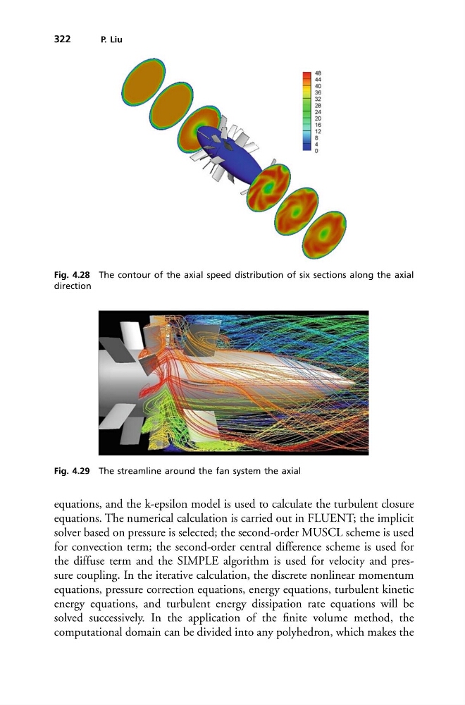
Fig. 4.28 The contour of the axial speed distribution of six sections along the axial
direction
Fig. 4.29 The streamline around the fan system the axial
equations, and the k-epsilon model is used to calculate the turbulent closure
equations. The numerical calculation is carried out in FLUENT; the implicit
solver based on pressure is selected; the second-order MUSCL scheme is used
for convection term; the second-order central difference scheme is used for
the diffuse term and the SIMPLE algorithm is used for velocity and pressure coupling. In the iterative calculation, the discrete nonlinear momentum
equations, pressure correction equations, energy equations, turbulent kinetic
energy equations, and turbulent energy dissipation rate equations will be
solved successively. In the application of the finite volume method, the
computational domain can be divided into any polyhedron, which makes the
P. Liu
Fig. 4.28 The contour of the axial speed distribution of six sections along the axial
direction
Fig. 4.29 The streamline around the fan system the axial
equations, and the k-epsilon model is used to calculate the turbulent closure
equations. The numerical calculation is carried out in FLUENT; the implicit
solver based on pressure is selected; the second-order MUSCL scheme is used
for convection term; the second-order central difference scheme is used for
the diffuse term and the SIMPLE algorithm is used for velocity and pressure coupling. In the iterative calculation, the discrete nonlinear momentum
equations, pressure correction equations, energy equations, turbulent kinetic
energy equations, and turbulent energy dissipation rate equations will be
solved successively. In the application of the finite volume method, the
computational domain can be divided into any polyhedron, which makes the