

316
P. Liu
4.5 Numerical Simulation of Flow Field
for a Large Axial Flow Fan
4.5.1 Problem Description
The numerical calculation process and results of a large axial flow fan with
a diameter of 12.35 m are presented in this example. The incompressible
N-S equations are used to calculate the full turbulent RANS equations, and
the k-epsilon model is used to calculate the turbulent closure equations. The
numerical calculation is carried out in FLUENT; the implicit solver based
on pressure is selected; the second-order MUSCL scheme is used for convection term; the second-order central difference scheme is used for diffuse term
and the simple algorithm is used for velocity and pressure coupling. In the
iterative calculation, the discrete nonlinear momentum equations, pressure
correction equations, energy equations, turbulent kinetic energy equations,
and turbulent energy dissipation rate equations will be solved successively.
In the application of the finite volume method, the computational domain
can be divided into any polyhedron, which makes the finite volume method
very convenient for mesh generation. The finite volume can be divided into
structural grid or unstructured grid. Structural grid is easy to construct highprecision discrete equations; unstructured grid is easy to generate, has strong
applicability. The combination of these two types of grid can also be used in
the simulation.
4.5.2 The Physical Model
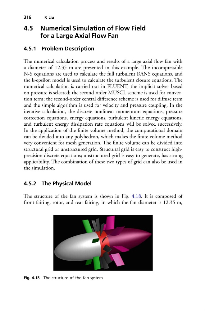
The structure of the fan system is shown in Fig. 4.18. It is composed of
front fairing, rotor, and rear fairing, in which the fan diameter is 12.35 m,
Fig. 4.18 The structure of the fan system
P. Liu
4.5 Numerical Simulation of Flow Field
for a Large Axial Flow Fan
4.5.1 Problem Description
The numerical calculation process and results of a large axial flow fan with
a diameter of 12.35 m are presented in this example. The incompressible
N-S equations are used to calculate the full turbulent RANS equations, and
the k-epsilon model is used to calculate the turbulent closure equations. The
numerical calculation is carried out in FLUENT; the implicit solver based
on pressure is selected; the second-order MUSCL scheme is used for convection term; the second-order central difference scheme is used for diffuse term
and the simple algorithm is used for velocity and pressure coupling. In the
iterative calculation, the discrete nonlinear momentum equations, pressure
correction equations, energy equations, turbulent kinetic energy equations,
and turbulent energy dissipation rate equations will be solved successively.
In the application of the finite volume method, the computational domain
can be divided into any polyhedron, which makes the finite volume method
very convenient for mesh generation. The finite volume can be divided into
structural grid or unstructured grid. Structural grid is easy to construct highprecision discrete equations; unstructured grid is easy to generate, has strong
applicability. The combination of these two types of grid can also be used in
the simulation.
4.5.2 The Physical Model
The structure of the fan system is shown in Fig. 4.18. It is composed of
front fairing, rotor, and rear fairing, in which the fan diameter is 12.35 m,
Fig. 4.18 The structure of the fan system