

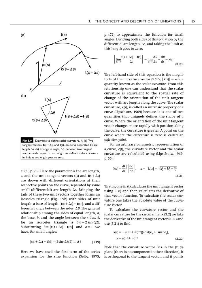
1969, p. 73). Here the parameter is the arc length,
s, and the unit tangent vectors t(s) and t(s ϩ⌬s)
are shown with different orientations at their
respective points on the curve, separated by some
small (differential) arc length ⌬s. Bringing the
tails of these two unit vectors together forms an
isosceles triangle (Fig. 3.9b) with sides of unit
length, a base of length |t(s ϩ⌬s) Ϫ t(s)|, and a differential angle between the sides, ⌬. The general
relationship among the sides of equal length, a,
the base, b, and the angle between the sides, ,
for an isosceles triangle is b/a ϭ 2 sin(/2).
Substituting b ϭ |t(sϩ⌬s) Ϫ t(s)| and a ϭ 1 we
have, for small angles:
(3.19)
Here we have used the first term of the series
expansion for the sine function (Selby, 1975,
|t(s ϩ ⌬s) Ϫ t(s)| ϭ 2 sin (⌬ր2) Х ⌬
p. 472) to approximate the function for small
angles. Dividing both sides of this equation by the
differential arc length, ⌬s, and taking the limit as
this length goes to zero:
(3.20)
The left-hand side of this equation is the magnitude of the curvature vector (3.17), |k(s)| ϭ (s), a
quantity known as the scalar curvature. From this
relationship one can understand that the scalar
curvature is equivalent to the spatial rate of
change of the orientation of the unit tangent
vector with arc length along the curve. The scalar
curvature, (s), is called an intrinsic property of a
curve (Lipschutz, 1969) because it is one of two
quantities that uniquely defines the shape of a
curve. Where the orientation of the unit tangent
vector changes more rapidly with position along
the curve, the curvature is greater. A point on the
curve where the curvature is zero is called an
inflection point.
For an arbitrary parametric representation of
a curve, c(t), the curvature vector and the scalar
curvature are calculated using (Lipschutz, 1969,
p. 65):
(3.21)
That is, one first calculates the unit tangent vector
using (3.8) and then calculates the derivative of
that vector function. To calculate the scalar curvature one takes the absolute value of the curvature vector.
To calculate the curvature vector and the
scalar curvature for the circular helix (3.2) we take
the derivative of the unit tangent vector (3.11) and
use (3.21) to find:
(3.22)
Note that the curvature vector lies in the (x, y)plane (there is no component in the z-direction), it
is orthogonal to the tangent vector, and it points
ϭ a(a 2 ϩ b 2 ) Ϫ1
k(t) ϭ Ϫa(a 2 ϩ b 2 ) Ϫ1 [(cos t)e x ϩ (sin t)e y ],
k(t) ϭ
dt
dt ր |
dc
dt | , ϭ |k(t)| ϭ √k 2
x ϩ k 2
y ϩ k 2
z
| lim
⌬s→0
t(s ϩ ⌬s) Ϫ t(s)
⌬s
| ϭ lim
⌬s→0
⌬
⌬s
ϭ
d
ds
ϭ (s)
3.1 THE CONCEPT AND DESCRIPTION OF LINEATIONS
85
Fig 3.9 Diagrams to define scalar curvature, . (a) Two
tangent vectors, t(s ϩ ⌬s) and t(s), on curve separated by arc
length ⌬s. (b) Change in angle, ⌬, between two tangent
vectors with respect to arc length ⌬s defines scalar curvature
in limit as arc length goes to zero.
x
y
z
(a)
(b)
⌬u
t(s)
c(s + ⌬s)
t(s + ⌬s)
t(s)
t (s + ⌬s)
t(s + ⌬s) – t(s)
c(s)
s, and the unit tangent vectors t(s) and t(s ϩ⌬s)
are shown with different orientations at their
respective points on the curve, separated by some
small (differential) arc length ⌬s. Bringing the
tails of these two unit vectors together forms an
isosceles triangle (Fig. 3.9b) with sides of unit
length, a base of length |t(s ϩ⌬s) Ϫ t(s)|, and a differential angle between the sides, ⌬. The general
relationship among the sides of equal length, a,
the base, b, and the angle between the sides, ,
for an isosceles triangle is b/a ϭ 2 sin(/2).
Substituting b ϭ |t(sϩ⌬s) Ϫ t(s)| and a ϭ 1 we
have, for small angles:
(3.19)
Here we have used the first term of the series
expansion for the sine function (Selby, 1975,
|t(s ϩ ⌬s) Ϫ t(s)| ϭ 2 sin (⌬ր2) Х ⌬
p. 472) to approximate the function for small
angles. Dividing both sides of this equation by the
differential arc length, ⌬s, and taking the limit as
this length goes to zero:
(3.20)
The left-hand side of this equation is the magnitude of the curvature vector (3.17), |k(s)| ϭ (s), a
quantity known as the scalar curvature. From this
relationship one can understand that the scalar
curvature is equivalent to the spatial rate of
change of the orientation of the unit tangent
vector with arc length along the curve. The scalar
curvature, (s), is called an intrinsic property of a
curve (Lipschutz, 1969) because it is one of two
quantities that uniquely defines the shape of a
curve. Where the orientation of the unit tangent
vector changes more rapidly with position along
the curve, the curvature is greater. A point on the
curve where the curvature is zero is called an
inflection point.
For an arbitrary parametric representation of
a curve, c(t), the curvature vector and the scalar
curvature are calculated using (Lipschutz, 1969,
p. 65):
(3.21)
That is, one first calculates the unit tangent vector
using (3.8) and then calculates the derivative of
that vector function. To calculate the scalar curvature one takes the absolute value of the curvature vector.
To calculate the curvature vector and the
scalar curvature for the circular helix (3.2) we take
the derivative of the unit tangent vector (3.11) and
use (3.21) to find:
(3.22)
Note that the curvature vector lies in the (x, y)plane (there is no component in the z-direction), it
is orthogonal to the tangent vector, and it points
ϭ a(a 2 ϩ b 2 ) Ϫ1
k(t) ϭ Ϫa(a 2 ϩ b 2 ) Ϫ1 [(cos t)e x ϩ (sin t)e y ],
k(t) ϭ
dt
dt ր |
dc
dt | , ϭ |k(t)| ϭ √k 2
x ϩ k 2
y ϩ k 2
z
| lim
⌬s→0
t(s ϩ ⌬s) Ϫ t(s)
⌬s
| ϭ lim
⌬s→0
⌬
⌬s
ϭ
d
ds
ϭ (s)
3.1 THE CONCEPT AND DESCRIPTION OF LINEATIONS
85
Fig 3.9 Diagrams to define scalar curvature, . (a) Two
tangent vectors, t(s ϩ ⌬s) and t(s), on curve separated by arc
length ⌬s. (b) Change in angle, ⌬, between two tangent
vectors with respect to arc length ⌬s defines scalar curvature
in limit as arc length goes to zero.
x
y
z
(a)
(b)
⌬u
t(s)
c(s + ⌬s)
t(s + ⌬s)
t(s)
t (s + ⌬s)
t(s + ⌬s) – t(s)
c(s)