

In the last step we used the fact that both vectors
have unit magnitude, so the product of their
absolute values is one. Solving for the angle :
(3.15)
As b goes to zero the helix collapses into a circle
on the (x, y)-plane and the angle goes to /2. This
special relationship is illustrated in Fig. 3.8b
where it is seen that t is perpendicular to the zaxis for all values of the arbitrary parameter t.
For a lineation observed at exposure, such as
the slickenlines in Fig. 3.3, the orientation determined in the field using geographic angles can be
related to the unit tangent vector, t. Although
slickenlines may be curved, they are approximated locally with linear elements whose orientation is measured using the plunge direction, ␣ p ,
and plunge, p . We assert that such a linear
element is parallel to the unit tangent vector of a
three-dimensional curve that passes through the
point of measurement, so it has the same direction angles. Furthermore, because t is a unit
vector, the scalar components are equivalent to
the direction cosines. We find using (2.101):
(3.16)
In this way we relate the orientation data taken at
scattered exposures on a continuous geological lineation to the components of the unit tangent
vectors at correlative points on a three-dimensional
curve.
As an example, consider the lineation
described by the plunge direction, ␣ p ϭ 222Њ, and
plunge, p ϭ 33Њ (Fig. 2.17). Substituting these
values into (3.16) we have t x ϭϪ0.561, t y ϭϪ0.623,
t z ϭϪ0.545 and |t| ϭ 1. Recall that the geographic coordinates (east, north, up) correspond
to the Cartesian coordinates (x, y, z), as shown in
Fig. 2.15, to reconcile the three negative components of the tangent vector with the orientation
of this lineation as plotted on the stereogram.
Also note that these components combine to give
a unit magnitude, as expected for the tangent
vector.
t x ϭ cos ␣ x ϭ sin ␣ p cos p
t y ϭ cos ␣ y ϭ cos ␣ p cos p
t z ϭ cos ␣ z ϭ Ϫ sin p
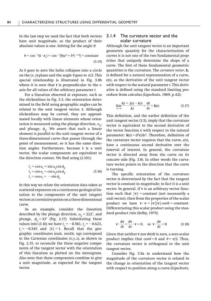
ϭ cos Ϫ1 (t · e z ) ϭ cos Ϫ1 [b(a 2 ϩ b 2 ) Ϫ1ր2 ] ϭ constant
3.1.4 The curvature vector and the
scalar curvature
Although the unit tangent vector is an important
geometric quantity for the characterization of
curves it is not one of the two fundamental properties that uniquely determine the shape of a
curve. The first of these fundamental geometric
quantities is the curvature. The curvature vector, k,
is defined for a natural representation of a curve,
c(s), as the derivative of the unit tangent vector
with respect to the natural parameter s. This derivative is defined using the standard limiting procedure from calculus (Lipschutz, 1969, p. 62):
(3.17)
This definition, and the earlier definition of the
unit tangent vector (3.5), imply that the curvature
vector is equivalent to the second derivative of
the vector function c with respect to the natural
parameter: k(s) ϭ d
2 c/ds
2 . Therefore, definition of
the curvature vector requires that the curve, c(s),
have a continuous second derivative over the
interval of interest. In general, the curvature
vector is directed away from the curve on its
concave side (Fig. 3.8). In other words the curvature vector points in the direction that the curve
is turning.
The specific orientation of the curvature
vector is determined by the fact that the tangent
vector is constant in magnitude; in fact it is a unit
vector. In general, if v is an arbitrary vector function such that |v| ϭ constant (not necessarily a
unit vector), then from the properties of the scalar
product we have
Differentiating this scalar product using the standard product rule (Selby, 1975):
(3.18)
Given that neither v nor dv/dt is zero, a zero scalar
product implies that cos ϭ 0 and ϭ /2. Thus,
the curvature vector is orthogonal to the unit
tangent vector.
Consider Fig. 3.9a to understand how the
magnitude of the curvature vector is related to
the change in orientation of the tangent vector
with respect to position along a curve (Lipschutz,
v ·
dv
dt
ϩ
dv
dt
· v ϭ 0, so v ·
dv
dt
ϭ 0
v · v ϭ |v||v| cos 0 ϭ constant.
lim
⌬s→0
t(s ϩ ⌬s) Ϫ t(s)
⌬s
ϭ
dt
ds
ϭ k(s)
84
CHARACTERIZING STRUCTURES USING DIFFERENTIAL GEOMETRY
have unit magnitude, so the product of their
absolute values is one. Solving for the angle :
(3.15)
As b goes to zero the helix collapses into a circle
on the (x, y)-plane and the angle goes to /2. This
special relationship is illustrated in Fig. 3.8b
where it is seen that t is perpendicular to the zaxis for all values of the arbitrary parameter t.
For a lineation observed at exposure, such as
the slickenlines in Fig. 3.3, the orientation determined in the field using geographic angles can be
related to the unit tangent vector, t. Although
slickenlines may be curved, they are approximated locally with linear elements whose orientation is measured using the plunge direction, ␣ p ,
and plunge, p . We assert that such a linear
element is parallel to the unit tangent vector of a
three-dimensional curve that passes through the
point of measurement, so it has the same direction angles. Furthermore, because t is a unit
vector, the scalar components are equivalent to
the direction cosines. We find using (2.101):
(3.16)
In this way we relate the orientation data taken at
scattered exposures on a continuous geological lineation to the components of the unit tangent
vectors at correlative points on a three-dimensional
curve.
As an example, consider the lineation
described by the plunge direction, ␣ p ϭ 222Њ, and
plunge, p ϭ 33Њ (Fig. 2.17). Substituting these
values into (3.16) we have t x ϭϪ0.561, t y ϭϪ0.623,
t z ϭϪ0.545 and |t| ϭ 1. Recall that the geographic coordinates (east, north, up) correspond
to the Cartesian coordinates (x, y, z), as shown in
Fig. 2.15, to reconcile the three negative components of the tangent vector with the orientation
of this lineation as plotted on the stereogram.
Also note that these components combine to give
a unit magnitude, as expected for the tangent
vector.
t x ϭ cos ␣ x ϭ sin ␣ p cos p
t y ϭ cos ␣ y ϭ cos ␣ p cos p
t z ϭ cos ␣ z ϭ Ϫ sin p
ϭ cos Ϫ1 (t · e z ) ϭ cos Ϫ1 [b(a 2 ϩ b 2 ) Ϫ1ր2 ] ϭ constant
3.1.4 The curvature vector and the
scalar curvature
Although the unit tangent vector is an important
geometric quantity for the characterization of
curves it is not one of the two fundamental properties that uniquely determine the shape of a
curve. The first of these fundamental geometric
quantities is the curvature. The curvature vector, k,
is defined for a natural representation of a curve,
c(s), as the derivative of the unit tangent vector
with respect to the natural parameter s. This derivative is defined using the standard limiting procedure from calculus (Lipschutz, 1969, p. 62):
(3.17)
This definition, and the earlier definition of the
unit tangent vector (3.5), imply that the curvature
vector is equivalent to the second derivative of
the vector function c with respect to the natural
parameter: k(s) ϭ d
2 c/ds
2 . Therefore, definition of
the curvature vector requires that the curve, c(s),
have a continuous second derivative over the
interval of interest. In general, the curvature
vector is directed away from the curve on its
concave side (Fig. 3.8). In other words the curvature vector points in the direction that the curve
is turning.
The specific orientation of the curvature
vector is determined by the fact that the tangent
vector is constant in magnitude; in fact it is a unit
vector. In general, if v is an arbitrary vector function such that |v| ϭ constant (not necessarily a
unit vector), then from the properties of the scalar
product we have
Differentiating this scalar product using the standard product rule (Selby, 1975):
(3.18)
Given that neither v nor dv/dt is zero, a zero scalar
product implies that cos ϭ 0 and ϭ /2. Thus,
the curvature vector is orthogonal to the unit
tangent vector.
Consider Fig. 3.9a to understand how the
magnitude of the curvature vector is related to
the change in orientation of the tangent vector
with respect to position along a curve (Lipschutz,
v ·
dv
dt
ϩ
dv
dt
· v ϭ 0, so v ·
dv
dt
ϭ 0
v · v ϭ |v||v| cos 0 ϭ constant.
lim
⌬s→0
t(s ϩ ⌬s) Ϫ t(s)
⌬s
ϭ
dt
ds
ϭ k(s)
84
CHARACTERIZING STRUCTURES USING DIFFERENTIAL GEOMETRY