

symbol for the arbitrary parameter of a curve, t,
from that for the unit tangent vector, t. This vector
is defined by considering the position vector to be
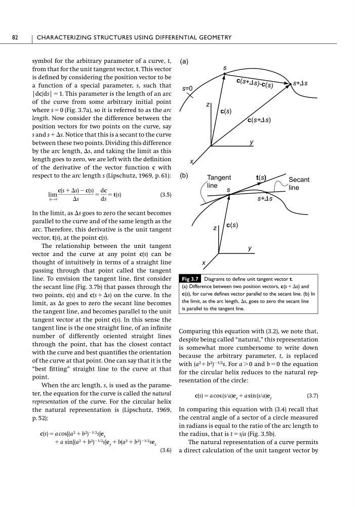
a function of a special parameter, s, such that
|dc/ds| ϭ 1. This parameter is the length of an arc
of the curve from some arbitrary initial point
where s ϭ 0 (Fig. 3.7a), so it is referred to as the arc
length. Now consider the difference between the
position vectors for two points on the curve, say
s and s ϩ⌬s. Notice that this is a secant to the curve
between these two points. Dividing this difference
by the arc length, ⌬s, and taking the limit as this
length goes to zero, we are left with the definition
of the derivative of the vector function c with
respect to the arc length s (Lipschutz, 1969, p. 61):
(3.5)
In the limit, as ⌬s goes to zero the secant becomes
parallel to the curve and of the same length as the
arc. Therefore, this derivative is the unit tangent
vector, t(s), at the point c(s).
The relationship between the unit tangent
vector and the curve at any point c(s) can be
thought of intuitively in terms of a straight line
passing through that point called the tangent
line. To envision the tangent line, first consider
the secant line (Fig. 3.7b) that passes through the
two points, c(s) and c(s ϩ⌬s) on the curve. In the
limit, as ⌬s goes to zero the secant line becomes
the tangent line, and becomes parallel to the unit
tangent vector at the point c(s). In this sense the
tangent line is the one straight line, of an infinite
number of differently oriented straight lines
through the point, that has the closest contact
with the curve and best quantifies the orientation
of the curve at that point. One can say that it is the
“best fitting” straight line to the curve at that
point.
When the arc length, s, is used as the parameter, the equation for the curve is called the natural
representation of the curve. For the circular helix
the natural representation is (Lipschutz, 1969,
p. 52):
(3.6)
ϩ a sin[(a 2 ϩ b 2 ) Ϫ1ր2 s]e y ϩ b(a 2 ϩ b 2 ) Ϫ1ր2 se z
c(s) ϭ a cos[(a 2 ϩ b 2 ) Ϫ1ր2 s]e x
lim
⌬s→0
c(s ϩ ⌬s) Ϫ c(s)
⌬s
ϭ
dc
ds
ϭ t(s)
Comparing this equation with (3.2), we note that,
despite being called “natural,” this representation
is somewhat more cumbersome to write down
because the arbitrary parameter, t, is replaced
with (a
2 ϩb
2 )
Ϫ1/2 s. For a Ͼ 0 and b ϭ 0 the equation
for the circular helix reduces to the natural representation of the circle:
(3.7)
In comparing this equation with (3.4) recall that
the central angle of a sector of a circle measured
in radians is equal to the ratio of the arc length to
the radius, that is t ϭ s/a (Fig. 3.5b).
The natural representation of a curve permits
a direct calculation of the unit tangent vector by
c(s) ϭ a cos (sրa)e x ϩ a sin (sրa)e y
82
CHARACTERIZING STRUCTURES USING DIFFERENTIAL GEOMETRY
Fig 3.7 Diagrams to define unit tangent vector t.
(a) Difference between two position vectors, c(s ϩ⌬s) and
c(s), for curve defines vector parallel to the secant line. (b) In
the limit, as the arc length, ⌬s, goes to zero the secant line
is parallel to the tangent line.
x
y
z
(a)
s
x
y
z
(b)
s
Tangent
line
Secant
line
s+⌬s
c(s)
c(s)
s+⌬s
c( s+ ⌬s )-c (s )
c(s+⌬s)
t(s)
s=0
from that for the unit tangent vector, t. This vector
is defined by considering the position vector to be
a function of a special parameter, s, such that
|dc/ds| ϭ 1. This parameter is the length of an arc
of the curve from some arbitrary initial point
where s ϭ 0 (Fig. 3.7a), so it is referred to as the arc
length. Now consider the difference between the
position vectors for two points on the curve, say
s and s ϩ⌬s. Notice that this is a secant to the curve
between these two points. Dividing this difference
by the arc length, ⌬s, and taking the limit as this
length goes to zero, we are left with the definition
of the derivative of the vector function c with
respect to the arc length s (Lipschutz, 1969, p. 61):
(3.5)
In the limit, as ⌬s goes to zero the secant becomes
parallel to the curve and of the same length as the
arc. Therefore, this derivative is the unit tangent
vector, t(s), at the point c(s).
The relationship between the unit tangent
vector and the curve at any point c(s) can be
thought of intuitively in terms of a straight line
passing through that point called the tangent
line. To envision the tangent line, first consider
the secant line (Fig. 3.7b) that passes through the
two points, c(s) and c(s ϩ⌬s) on the curve. In the
limit, as ⌬s goes to zero the secant line becomes
the tangent line, and becomes parallel to the unit
tangent vector at the point c(s). In this sense the
tangent line is the one straight line, of an infinite
number of differently oriented straight lines
through the point, that has the closest contact
with the curve and best quantifies the orientation
of the curve at that point. One can say that it is the
“best fitting” straight line to the curve at that
point.
When the arc length, s, is used as the parameter, the equation for the curve is called the natural
representation of the curve. For the circular helix
the natural representation is (Lipschutz, 1969,
p. 52):
(3.6)
ϩ a sin[(a 2 ϩ b 2 ) Ϫ1ր2 s]e y ϩ b(a 2 ϩ b 2 ) Ϫ1ր2 se z
c(s) ϭ a cos[(a 2 ϩ b 2 ) Ϫ1ր2 s]e x
lim
⌬s→0
c(s ϩ ⌬s) Ϫ c(s)
⌬s
ϭ
dc
ds
ϭ t(s)
Comparing this equation with (3.2), we note that,
despite being called “natural,” this representation
is somewhat more cumbersome to write down
because the arbitrary parameter, t, is replaced
with (a
2 ϩb
2 )
Ϫ1/2 s. For a Ͼ 0 and b ϭ 0 the equation
for the circular helix reduces to the natural representation of the circle:
(3.7)
In comparing this equation with (3.4) recall that
the central angle of a sector of a circle measured
in radians is equal to the ratio of the arc length to
the radius, that is t ϭ s/a (Fig. 3.5b).
The natural representation of a curve permits
a direct calculation of the unit tangent vector by
c(s) ϭ a cos (sրa)e x ϩ a sin (sրa)e y
82
CHARACTERIZING STRUCTURES USING DIFFERENTIAL GEOMETRY
Fig 3.7 Diagrams to define unit tangent vector t.
(a) Difference between two position vectors, c(s ϩ⌬s) and
c(s), for curve defines vector parallel to the secant line. (b) In
the limit, as the arc length, ⌬s, goes to zero the secant line
is parallel to the tangent line.
x
y
z
(a)
s
x
y
z
(b)
s
Tangent
line
Secant
line
s+⌬s
c(s)
c(s)
s+⌬s
c( s+ ⌬s )-c (s )
c(s+⌬s)
t(s)
s=0