

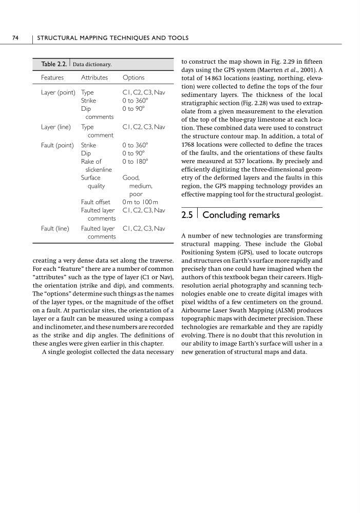
creating a very dense data set along the traverse.
For each “feature” there are a number of common
“attributes” such as the type of layer (C1 or Nav),
the orientation (strike and dip), and comments.
The “options” determine such things as the names
of the layer types, or the magnitude of the offset
on a fault. At particular sites, the orientation of a
layer or a fault can be measured using a compass
and inclinometer, and these numbers are recorded
as the strike and dip angles. The definitions of
these angles were given earlier in this chapter.
A single geologist collected the data necessary
to construct the map shown in Fig. 2.29 in fifteen
days using the GPS system (Maerten et al., 2001). A
total of 14 863 locations (easting, northing, elevation) were collected to define the tops of the four
sedimentary layers. The thickness of the local
stratigraphic section (Fig. 2.28) was used to extrapolate from a given measurement to the elevation
of the top of the blue-gray limestone at each location. These combined data were used to construct
the structure contour map. In addition, a total of
1768 locations were collected to define the traces
of the faults, and the orientations of these faults
were measured at 537 locations. By precisely and
efficiently digitizing the three-dimensional geometry of the deformed layers and the faults in this
region, the GPS mapping technology provides an
effective mapping tool for the structural geologist.
2.5 Concluding remarks
A number of new technologies are transforming
structural mapping. These include the Global
Positioning System (GPS), used to locate outcrops
and structures on Earth’s surface more rapidly and
precisely than one could have imagined when the
authors of this textbook began their careers. Highresolution aerial photography and scanning technologies enable one to create digital images with
pixel widths of a few centimeters on the ground.
Airbourne Laser Swath Mapping (ALSM) produces
topographic maps with decimeter precision. These
technologies are remarkable and they are rapidly
evolving. There is no doubt that this revolution in
our ability to image Earth’s surface will usher in a
new generation of structural maps and data.
74
STRUCTURAL MAPPING TECHNIQUES AND TOOLS
Table 2.2. Data dictionary.
Features
Attributes
Options
Layer (point) Type
C1, C2, C3, Nav
Strike
0 to 360Њ
Dip
0 to 90Њ
comments
Layer (line)
Type
C1, C2, C3, Nav
comment
Fault (point) Strike
0 to 360Њ
Dip
0 to 90Њ
Rake of
0 to 180Њ
slickenline
Surface
Good,
quality
medium,
poor
Fault offset
0 m to 100 m
Faulted layer C1, C2, C3, Nav
comments
Fault (line)
Faulted layer C1, C2, C3, Nav
comments
For each “feature” there are a number of common
“attributes” such as the type of layer (C1 or Nav),
the orientation (strike and dip), and comments.
The “options” determine such things as the names
of the layer types, or the magnitude of the offset
on a fault. At particular sites, the orientation of a
layer or a fault can be measured using a compass
and inclinometer, and these numbers are recorded
as the strike and dip angles. The definitions of
these angles were given earlier in this chapter.
A single geologist collected the data necessary
to construct the map shown in Fig. 2.29 in fifteen
days using the GPS system (Maerten et al., 2001). A
total of 14 863 locations (easting, northing, elevation) were collected to define the tops of the four
sedimentary layers. The thickness of the local
stratigraphic section (Fig. 2.28) was used to extrapolate from a given measurement to the elevation
of the top of the blue-gray limestone at each location. These combined data were used to construct
the structure contour map. In addition, a total of
1768 locations were collected to define the traces
of the faults, and the orientations of these faults
were measured at 537 locations. By precisely and
efficiently digitizing the three-dimensional geometry of the deformed layers and the faults in this
region, the GPS mapping technology provides an
effective mapping tool for the structural geologist.
2.5 Concluding remarks
A number of new technologies are transforming
structural mapping. These include the Global
Positioning System (GPS), used to locate outcrops
and structures on Earth’s surface more rapidly and
precisely than one could have imagined when the
authors of this textbook began their careers. Highresolution aerial photography and scanning technologies enable one to create digital images with
pixel widths of a few centimeters on the ground.
Airbourne Laser Swath Mapping (ALSM) produces
topographic maps with decimeter precision. These
technologies are remarkable and they are rapidly
evolving. There is no doubt that this revolution in
our ability to image Earth’s surface will usher in a
new generation of structural maps and data.
74
STRUCTURAL MAPPING TECHNIQUES AND TOOLS
Table 2.2. Data dictionary.
Features
Attributes
Options
Layer (point) Type
C1, C2, C3, Nav
Strike
0 to 360Њ
Dip
0 to 90Њ
comments
Layer (line)
Type
C1, C2, C3, Nav
comment
Fault (point) Strike
0 to 360Њ
Dip
0 to 90Њ
Rake of
0 to 180Њ
slickenline
Surface
Good,
quality
medium,
poor
Fault offset
0 m to 100 m
Faulted layer C1, C2, C3, Nav
comments
Fault (line)
Faulted layer C1, C2, C3, Nav
comments