

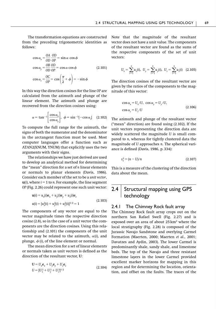
The transformation equations are constructed
from the preceding trigonometric identities as
follows:
(2.101)
In this way the direction cosines for the line OP are
calculated from the azimuth and plunge of the
linear element. The azimuth and plunge are
recovered from the direction cosines using:
(2.102)
To compute the full range for the azimuth, the
signs of both the numerator and the denominator
in the arctangent function must be used. Most
computer languages offer a function such as
ATAN2(XNUM, YNUM) that explicitly uses the two
arguments with their signs.
The relationships we have just derived are used
to develop an analytical method for determining
the “mean” direction for a set of n linear elements
or normals to planar elements (Davis, 1986).
Consider each member of the set to be a unit vector,
u(i), where i ϭ 1 to n. For example, the line segment
OP (Fig. 2.26) could represent one such unit vector:
(2.103)
The components of any vector are equal to the
vector magnitude times the respective direction
cosine (2.8), so in the case of a unit vector the components are the direction cosines. Using this relationship and (2.101) the components of the unit
vector may be related to the azimuth, ␣(i), and
plunge, (i), of the line element or normal.
The mean direction for a set of linear elements
or normals taken as unit vectors is defined as the
direction of the resultant vector, U:
(2.104)
U ϭ [U 2
x ϩ U 2
y ϩ U 2
z ] 1ր2
U ϭ U x e x ϩ U y e y ϩ U z e z
u(i) ϭ [u 2
x (i) ϩ u 2
y (i) ϩ u 2
z (i)] 1ր2 ϭ 1
u(i) ϭ u x (i)e x ϩ u y (i)e y ϩ u z (i)e z
␣ ϭ tan Ϫ1
΄
cos ␣ x
cos ␣ y ΅ , ϭ sin Ϫ1 [Ϫcos ␣ z ]
cos ␣ z ϭ
OC
OP
ϭ cos
2
ϩ ϭ Ϫ sin
cos ␣ y ϭ
OB
OD
OD
OP
ϭ cos ␣ cos
cos ␣ x ϭ
OA
OD
OD
OP
ϭ sin ␣ cos
Note that the magnitude of the resultant
vector does not have a unit value. The components
of the resultant vector are found as the sums of
the respective components of the set of unit
vectors:
(2.105)
The direction cosines of the resultant vector are
given by the ratios of the components to the magnitude of this vector:
(2.106)
The azimuth and plunge of the resultant vector
(“mean” direction) are found using (2.102). If the
unit vectors representing the direction data are
widely scattered the magnitude U is small compared to n, whereas for tightly clustered data the
magnitude of U approaches n. The spherical variance is defined (Davis, 1986, p. 334):
(2.107)
This is a measure of the clustering of the direction
data about the mean.
2.4 Structural mapping using GPS
technology
2.4.1 The Chimney Rock fault array
The Chimney Rock fault array crops out on the
northern San Rafael Swell (Fig. 2.27) and is
exposed over an area of about 25 km
2 where the
local stratigraphy (Fig. 2.28) is composed of the
Jurassic Navajo Sandstone and overlying Carmel
Formation (Maerten, 2000; Maerten et al., 2001;
Davatzes and Aydin, 2003). The lower Carmel is
predominantly shale, sandy shale, and limestone
beds. The top of the Navajo and three resistant
limestone layers in the lower Carmel provided
excellent marker horizons for mapping in this
region and for determining the location, orientation, and offset on the faults. The traces of the
s 2
s ϭ (n Ϫ U)րn
cos ␣ z ϭ U z րU
cos ␣ x ϭ U x րU, cos ␣ y ϭ U y րU,
U x ϭ ͚
n
iϭ1
u x (i), U y ϭ ͚
n
iϭ1
u y (i), U z ϭ ͚
n
iϭ1
u z (i)
2.4 STRUCTURAL MAPPING USING GPS TECHNOLOGY
69
from the preceding trigonometric identities as
follows:
(2.101)
In this way the direction cosines for the line OP are
calculated from the azimuth and plunge of the
linear element. The azimuth and plunge are
recovered from the direction cosines using:
(2.102)
To compute the full range for the azimuth, the
signs of both the numerator and the denominator
in the arctangent function must be used. Most
computer languages offer a function such as
ATAN2(XNUM, YNUM) that explicitly uses the two
arguments with their signs.
The relationships we have just derived are used
to develop an analytical method for determining
the “mean” direction for a set of n linear elements
or normals to planar elements (Davis, 1986).
Consider each member of the set to be a unit vector,
u(i), where i ϭ 1 to n. For example, the line segment
OP (Fig. 2.26) could represent one such unit vector:
(2.103)
The components of any vector are equal to the
vector magnitude times the respective direction
cosine (2.8), so in the case of a unit vector the components are the direction cosines. Using this relationship and (2.101) the components of the unit
vector may be related to the azimuth, ␣(i), and
plunge, (i), of the line element or normal.
The mean direction for a set of linear elements
or normals taken as unit vectors is defined as the
direction of the resultant vector, U:
(2.104)
U ϭ [U 2
x ϩ U 2
y ϩ U 2
z ] 1ր2
U ϭ U x e x ϩ U y e y ϩ U z e z
u(i) ϭ [u 2
x (i) ϩ u 2
y (i) ϩ u 2
z (i)] 1ր2 ϭ 1
u(i) ϭ u x (i)e x ϩ u y (i)e y ϩ u z (i)e z
␣ ϭ tan Ϫ1
΄
cos ␣ x
cos ␣ y ΅ , ϭ sin Ϫ1 [Ϫcos ␣ z ]
cos ␣ z ϭ
OC
OP
ϭ cos
2
ϩ ϭ Ϫ sin
cos ␣ y ϭ
OB
OD
OD
OP
ϭ cos ␣ cos
cos ␣ x ϭ
OA
OD
OD
OP
ϭ sin ␣ cos
Note that the magnitude of the resultant
vector does not have a unit value. The components
of the resultant vector are found as the sums of
the respective components of the set of unit
vectors:
(2.105)
The direction cosines of the resultant vector are
given by the ratios of the components to the magnitude of this vector:
(2.106)
The azimuth and plunge of the resultant vector
(“mean” direction) are found using (2.102). If the
unit vectors representing the direction data are
widely scattered the magnitude U is small compared to n, whereas for tightly clustered data the
magnitude of U approaches n. The spherical variance is defined (Davis, 1986, p. 334):
(2.107)
This is a measure of the clustering of the direction
data about the mean.
2.4 Structural mapping using GPS
technology
2.4.1 The Chimney Rock fault array
The Chimney Rock fault array crops out on the
northern San Rafael Swell (Fig. 2.27) and is
exposed over an area of about 25 km
2 where the
local stratigraphy (Fig. 2.28) is composed of the
Jurassic Navajo Sandstone and overlying Carmel
Formation (Maerten, 2000; Maerten et al., 2001;
Davatzes and Aydin, 2003). The lower Carmel is
predominantly shale, sandy shale, and limestone
beds. The top of the Navajo and three resistant
limestone layers in the lower Carmel provided
excellent marker horizons for mapping in this
region and for determining the location, orientation, and offset on the faults. The traces of the
s 2
s ϭ (n Ϫ U)րn
cos ␣ z ϭ U z րU
cos ␣ x ϭ U x րU, cos ␣ y ϭ U y րU,
U x ϭ ͚
n
iϭ1
u x (i), U y ϭ ͚
n
iϭ1
u y (i), U z ϭ ͚
n
iϭ1
u z (i)
2.4 STRUCTURAL MAPPING USING GPS TECHNOLOGY
69