

with a rake of 116 lying in a planar element with
strike and dip of (064, 58).
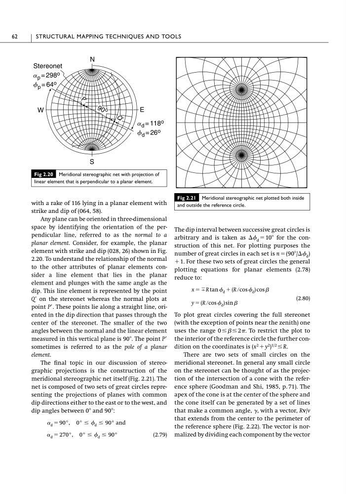
Any plane can be oriented in three-dimensional
space by identifying the orientation of the perpendicular line, referred to as the normal to a
planar element. Consider, for example, the planar
element with strike and dip (028, 26) shown in Fig.
2.20. To understand the relationship of the normal
to the other attributes of planar elements consider a line element that lies in the planar
element and plunges with the same angle as the
dip. This line element is represented by the point
Q� on the stereonet whereas the normal plots at
point P�. These points lie along a straight line, oriented in the dip direction that passes through the
center of the stereonet. The smaller of the two
angles between the normal and the linear element
measured in this vertical plane is 90�. The point P�
sometimes is referred to as the pole of a planar
element.
The final topic in our discussion of stereographic projections is the construction of the
meridional stereographic net itself (Fig. 2.21). The
net is composed of two sets of great circles representing the projections of planes with common
dip directions either to the east or to the west, and
dip angles between 0� and 90�:
(2.79)
� d � 270°, 0° � � d � 90°
� d � 90°, 0° � � d � 90° and
The dip interval between successive great circles is
arbitrary and is taken as �� d � 10� for the construction of this net. For plotting purposes the
number of great circles in each set is n � (90�/�� d )
� 1. For these two sets of great circles the general
plotting equations for planar elements (2.78)
reduce to:
(2.80)
To plot great circles covering the full stereonet
(with the exception of points near the zenith) one
uses the range 0 � � � 2�. To restrict the plot to
the interior of the reference circle the further condition on the coordinates is (x
2 � y
2 )
1/2 � R.
There are two sets of small circles on the
meridional stereonet. In general any small circle
on the stereonet can be thought of as the projection of the intersection of a cone with the reference sphere (Goodman and Shi, 1985, p. 71). The
apex of the cone is at the center of the sphere and
the cone itself can be generated by a set of lines
that make a common angle, �, with a vector, Rv/v
that extends from the center to the perimeter of
the reference sphere (Fig. 2.22). The vector is normalized by dividing each component by the vector
y � (R �cos � d ) sin �
x � �R tan � d � (R �cos � d ) cos �
62
STRUCTURAL MAPPING TECHNIQUES AND TOOLS
Fig 2.20 Meridional stereographic net with projection of
linear element that is perpendicular to a planar element.
N
W
S
E
Q �
P �
Stereonet
a p = 298 o
f p = 64 o
9 0 o
a d = 118 o
f d = 26 o
Fig 2.21 Meridional stereographic net plotted both inside
and outside the reference circle.
strike and dip of (064, 58).
Any plane can be oriented in three-dimensional
space by identifying the orientation of the perpendicular line, referred to as the normal to a
planar element. Consider, for example, the planar
element with strike and dip (028, 26) shown in Fig.
2.20. To understand the relationship of the normal
to the other attributes of planar elements consider a line element that lies in the planar
element and plunges with the same angle as the
dip. This line element is represented by the point
Q� on the stereonet whereas the normal plots at
point P�. These points lie along a straight line, oriented in the dip direction that passes through the
center of the stereonet. The smaller of the two
angles between the normal and the linear element
measured in this vertical plane is 90�. The point P�
sometimes is referred to as the pole of a planar
element.
The final topic in our discussion of stereographic projections is the construction of the
meridional stereographic net itself (Fig. 2.21). The
net is composed of two sets of great circles representing the projections of planes with common
dip directions either to the east or to the west, and
dip angles between 0� and 90�:
(2.79)
� d � 270°, 0° � � d � 90°
� d � 90°, 0° � � d � 90° and
The dip interval between successive great circles is
arbitrary and is taken as �� d � 10� for the construction of this net. For plotting purposes the
number of great circles in each set is n � (90�/�� d )
� 1. For these two sets of great circles the general
plotting equations for planar elements (2.78)
reduce to:
(2.80)
To plot great circles covering the full stereonet
(with the exception of points near the zenith) one
uses the range 0 � � � 2�. To restrict the plot to
the interior of the reference circle the further condition on the coordinates is (x
2 � y
2 )
1/2 � R.
There are two sets of small circles on the
meridional stereonet. In general any small circle
on the stereonet can be thought of as the projection of the intersection of a cone with the reference sphere (Goodman and Shi, 1985, p. 71). The
apex of the cone is at the center of the sphere and
the cone itself can be generated by a set of lines
that make a common angle, �, with a vector, Rv/v
that extends from the center to the perimeter of
the reference sphere (Fig. 2.22). The vector is normalized by dividing each component by the vector
y � (R �cos � d ) sin �
x � �R tan � d � (R �cos � d ) cos �
62
STRUCTURAL MAPPING TECHNIQUES AND TOOLS
Fig 2.20 Meridional stereographic net with projection of
linear element that is perpendicular to a planar element.
N
W
S
E
Q �
P �
Stereonet
a p = 298 o
f p = 64 o
9 0 o
a d = 118 o
f d = 26 o
Fig 2.21 Meridional stereographic net plotted both inside
and outside the reference circle.