

direction cosines, m ij . These three quantities may
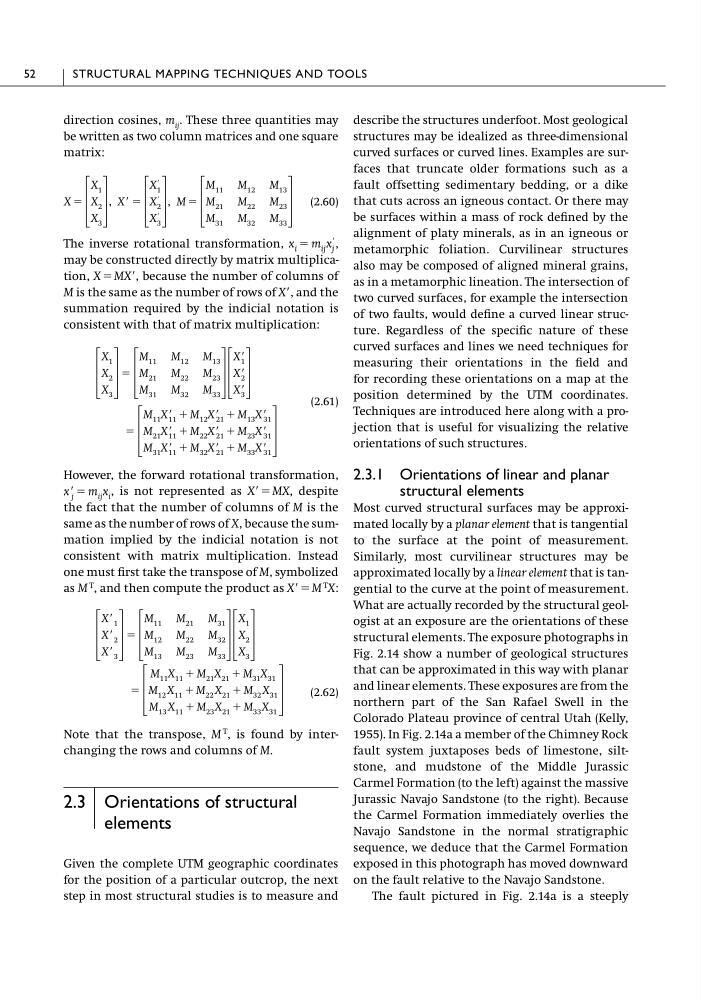
be written as two column matrices and one square
matrix:
(2.60)
The inverse rotational transformation,
,
may be constructed directly by matrix multiplication, X ϭ MXЈ, because the number of columns of
M is the same as the number of rows of XЈ, and the
summation required by the indicial notation is
consistent with that of matrix multiplication:
(2.61)
However, the forward rotational transformation,
, is not represented as XЈϭMX, despite
the fact that the number of columns of M is the
same as the number of rows of X, because the summation implied by the indicial notation is not
consistent with matrix multiplication. Instead
one must first take the transpose of M, symbolized
as M
T , and then compute the product as XЈϭM
T X:
(2.62)
Note that the transpose, M
T , is found by interchanging the rows and columns of M.
2.3 Orientations of structural
elements
Given the complete UTM geographic coordinates
for the position of a particular outcrop, the next
step in most structural studies is to measure and
ϭ
΄
M 11 X 11 ϩ M 21 X 21 ϩ M 31 X 31
M 12 X 11 ϩ M 22 X 21 ϩ M 32 X 31
M 13 X 11 ϩ M 23 X 21 ϩ M 33 X 31
΅
΄
XЈ 1
XЈ 2
XЈ 3
΅
ϭ
΄
M 11 M 21 M 31
M 12 M 22 M 32
M 13 M 23 M 33
΅΄
X 1
X 2
X 3
΅
xЈ j ϭ m ij x i
ϭ
΄
M 11 XЈ 11 ϩ M 12 XЈ 21 ϩ M 13 XЈ 31
M 21 XЈ 11 ϩ M 22 XЈ 21 ϩ M 23 XЈ 31
M 31 XЈ 11 ϩ M 32 XЈ 21 ϩ M 33 XЈ 31
΅
΄
X 1
X 2
X 3
΅
ϭ
΄
M 11 M 12 M 13
M 21 M 22 M 23
M 31 M 32 M 33
΅΄
XЈ 1
XЈ 2
XЈ 3
΅
x i ϭ m ij x Ј
j
X ϭ
΄
X 1
X 2
X 3
΅
, XЈ ϭ
΄
X Ј
1
X Ј
2
X Ј
3
΅
, M ϭ
΄
M 11 M 12 M 13
M 21 M 22 M 23
M 31 M 32 M 33
΅
describe the structures underfoot. Most geological
structures may be idealized as three-dimensional
curved surfaces or curved lines. Examples are surfaces that truncate older formations such as a
fault offsetting sedimentary bedding, or a dike
that cuts across an igneous contact. Or there may
be surfaces within a mass of rock defined by the
alignment of platy minerals, as in an igneous or
metamorphic foliation. Curvilinear structures
also may be composed of aligned mineral grains,
as in a metamorphic lineation. The intersection of
two curved surfaces, for example the intersection
of two faults, would define a curved linear structure. Regardless of the specific nature of these
curved surfaces and lines we need techniques for
measuring their orientations in the field and
for recording these orientations on a map at the
position determined by the UTM coordinates.
Techniques are introduced here along with a projection that is useful for visualizing the relative
orientations of such structures.
2.3.1 Orientations of linear and planar
structural elements
Most curved structural surfaces may be approximated locally by a planar element that is tangential
to the surface at the point of measurement.
Similarly, most curvilinear structures may be
approximated locally by a linear element that is tangential to the curve at the point of measurement.
What are actually recorded by the structural geologist at an exposure are the orientations of these
structural elements. The exposure photographs in
Fig. 2.14 show a number of geological structures
that can be approximated in this way with planar
and linear elements. These exposures are from the
northern part of the San Rafael Swell in the
Colorado Plateau province of central Utah (Kelly,
1955). In Fig. 2.14a a member of the Chimney Rock
fault system juxtaposes beds of limestone, siltstone, and mudstone of the Middle Jurassic
Carmel Formation (to the left) against the massive
Jurassic Navajo Sandstone (to the right). Because
the Carmel Formation immediately overlies the
Navajo Sandstone in the normal stratigraphic
sequence, we deduce that the Carmel Formation
exposed in this photograph has moved downward
on the fault relative to the Navajo Sandstone.
The fault pictured in Fig. 2.14a is a steeply
52
STRUCTURAL MAPPING TECHNIQUES AND TOOLS
be written as two column matrices and one square
matrix:
(2.60)
The inverse rotational transformation,
,
may be constructed directly by matrix multiplication, X ϭ MXЈ, because the number of columns of
M is the same as the number of rows of XЈ, and the
summation required by the indicial notation is
consistent with that of matrix multiplication:
(2.61)
However, the forward rotational transformation,
, is not represented as XЈϭMX, despite
the fact that the number of columns of M is the
same as the number of rows of X, because the summation implied by the indicial notation is not
consistent with matrix multiplication. Instead
one must first take the transpose of M, symbolized
as M
T , and then compute the product as XЈϭM
T X:
(2.62)
Note that the transpose, M
T , is found by interchanging the rows and columns of M.
2.3 Orientations of structural
elements
Given the complete UTM geographic coordinates
for the position of a particular outcrop, the next
step in most structural studies is to measure and
ϭ
΄
M 11 X 11 ϩ M 21 X 21 ϩ M 31 X 31
M 12 X 11 ϩ M 22 X 21 ϩ M 32 X 31
M 13 X 11 ϩ M 23 X 21 ϩ M 33 X 31
΅
΄
XЈ 1
XЈ 2
XЈ 3
΅
ϭ
΄
M 11 M 21 M 31
M 12 M 22 M 32
M 13 M 23 M 33
΅΄
X 1
X 2
X 3
΅
xЈ j ϭ m ij x i
ϭ
΄
M 11 XЈ 11 ϩ M 12 XЈ 21 ϩ M 13 XЈ 31
M 21 XЈ 11 ϩ M 22 XЈ 21 ϩ M 23 XЈ 31
M 31 XЈ 11 ϩ M 32 XЈ 21 ϩ M 33 XЈ 31
΅
΄
X 1
X 2
X 3
΅
ϭ
΄
M 11 M 12 M 13
M 21 M 22 M 23
M 31 M 32 M 33
΅΄
XЈ 1
XЈ 2
XЈ 3
΅
x i ϭ m ij x Ј
j
X ϭ
΄
X 1
X 2
X 3
΅
, XЈ ϭ
΄
X Ј
1
X Ј
2
X Ј
3
΅
, M ϭ
΄
M 11 M 12 M 13
M 21 M 22 M 23
M 31 M 32 M 33
΅
describe the structures underfoot. Most geological
structures may be idealized as three-dimensional
curved surfaces or curved lines. Examples are surfaces that truncate older formations such as a
fault offsetting sedimentary bedding, or a dike
that cuts across an igneous contact. Or there may
be surfaces within a mass of rock defined by the
alignment of platy minerals, as in an igneous or
metamorphic foliation. Curvilinear structures
also may be composed of aligned mineral grains,
as in a metamorphic lineation. The intersection of
two curved surfaces, for example the intersection
of two faults, would define a curved linear structure. Regardless of the specific nature of these
curved surfaces and lines we need techniques for
measuring their orientations in the field and
for recording these orientations on a map at the
position determined by the UTM coordinates.
Techniques are introduced here along with a projection that is useful for visualizing the relative
orientations of such structures.
2.3.1 Orientations of linear and planar
structural elements
Most curved structural surfaces may be approximated locally by a planar element that is tangential
to the surface at the point of measurement.
Similarly, most curvilinear structures may be
approximated locally by a linear element that is tangential to the curve at the point of measurement.
What are actually recorded by the structural geologist at an exposure are the orientations of these
structural elements. The exposure photographs in
Fig. 2.14 show a number of geological structures
that can be approximated in this way with planar
and linear elements. These exposures are from the
northern part of the San Rafael Swell in the
Colorado Plateau province of central Utah (Kelly,
1955). In Fig. 2.14a a member of the Chimney Rock
fault system juxtaposes beds of limestone, siltstone, and mudstone of the Middle Jurassic
Carmel Formation (to the left) against the massive
Jurassic Navajo Sandstone (to the right). Because
the Carmel Formation immediately overlies the
Navajo Sandstone in the normal stratigraphic
sequence, we deduce that the Carmel Formation
exposed in this photograph has moved downward
on the fault relative to the Navajo Sandstone.
The fault pictured in Fig. 2.14a is a steeply
52
STRUCTURAL MAPPING TECHNIQUES AND TOOLS