

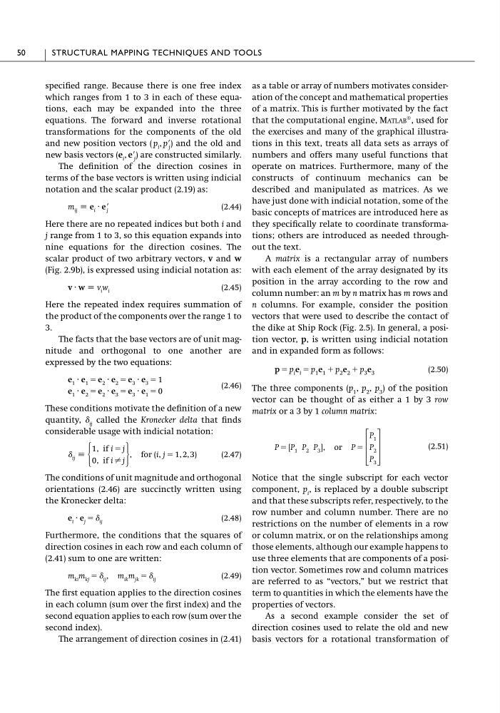
specified range. Because there is one free index
which ranges from 1 to 3 in each of these equations, each may be expanded into the three
equations. The forward and inverse rotational
transformations for the components of the old
and new position vectors
and the old and
new basis vectors
are constructed similarly.
The definition of the direction cosines in
terms of the base vectors is written using indicial
notation and the scalar product (2.19) as:
(2.44)
Here there are no repeated indices but both i and
j range from 1 to 3, so this equation expands into
nine equations for the direction cosines. The
scalar product of two arbitrary vectors, v and w
(Fig. 2.9b), is expressed using indicial notation as:
(2.45)
Here the repeated index requires summation of
the product of the components over the range 1 to
3.
The facts that the base vectors are of unit magnitude and orthogonal to one another are
expressed by the two equations:
(2.46)
These conditions motivate the definition of a new
quantity, ␦ ij called the Kronecker delta that finds
considerable usage with indicial notation:
(2.47)
The conditions of unit magnitude and orthogonal
orientations (2.46) are succinctly written using
the Kronecker delta:
(2.48)
Furthermore, the conditions that the squares of
direction cosines in each row and each column of
(2.41) sum to one are written:
(2.49)
The first equation applies to the direction cosines
in each column (sum over the first index) and the
second equation applies to each row (sum over the
second index).
The arrangement of direction cosines in (2.41)
m ki m kj ϭ ␦ ij , m ik m jk ϭ ␦ ij
e i · e j ϭ ␦ ij
␦ ij ϵ Ά
1, if i ϭ j
0, if i ϶ j ·
, for (i, j ϭ 1, 2, 3)
e 1 · e 2 ϭ e 2 · e 3 ϭ e 3 · e 1 ϭ 0
e 1 · e 1 ϭ e 2 · e 2 ϭ e 3 · e 3 ϭ 1
v · w ϵ v i w i
m ij ϵ e i · eЈ j
(e i , eЈ j )
( p i , pЈ j )
as a table or array of numbers motivates consideration of the concept and mathematical properties
of a matrix. This is further motivated by the fact
that the computational engine, MATLAB®, used for
the exercises and many of the graphical illustrations in this text, treats all data sets as arrays of
numbers and offers many useful functions that
operate on matrices. Furthermore, many of the
constructs of continuum mechanics can be
described and manipulated as matrices. As we
have just done with indicial notation, some of the
basic concepts of matrices are introduced here as
they specifically relate to coordinate transformations; others are introduced as needed throughout the text.
A matrix is a rectangular array of numbers
with each element of the array designated by its
position in the array according to the row and
column number: an m by n matrix has m rows and
n columns. For example, consider the position
vectors that were used to describe the contact of
the dike at Ship Rock (Fig. 2.5). In general, a position vector, p, is written using indicial notation
and in expanded form as follows:
(2.50)
The three components (p 1 , p 2 , p 3 ) of the position
vector can be thought of as either a 1 by 3 row
matrix or a 3 by 1 column matrix:
(2.51)
Notice that the single subscript for each vector
component, p i , is replaced by a double subscript
and that these subscripts refer, respectively, to the
row number and column number. There are no
restrictions on the number of elements in a row
or column matrix, or on the relationships among
those elements, although our example happens to
use three elements that are components of a position vector. Sometimes row and column matrices
are referred to as “vectors,” but we restrict that
term to quantities in which the elements have the
properties of vectors.
As a second example consider the set of
direction cosines used to relate the old and new
basis vectors for a rotational transformation of
P ϭ [P 1 P 2 P 3 ], or P ϭ
΄
P 1
P 2
P 3
΅
p ϭ p i e i ϭ p 1 e 1 ϩ p 2 e 2 ϩ p 3 e 3
50
STRUCTURAL MAPPING TECHNIQUES AND TOOLS
which ranges from 1 to 3 in each of these equations, each may be expanded into the three
equations. The forward and inverse rotational
transformations for the components of the old
and new position vectors
and the old and
new basis vectors
are constructed similarly.
The definition of the direction cosines in
terms of the base vectors is written using indicial
notation and the scalar product (2.19) as:
(2.44)
Here there are no repeated indices but both i and
j range from 1 to 3, so this equation expands into
nine equations for the direction cosines. The
scalar product of two arbitrary vectors, v and w
(Fig. 2.9b), is expressed using indicial notation as:
(2.45)
Here the repeated index requires summation of
the product of the components over the range 1 to
3.
The facts that the base vectors are of unit magnitude and orthogonal to one another are
expressed by the two equations:
(2.46)
These conditions motivate the definition of a new
quantity, ␦ ij called the Kronecker delta that finds
considerable usage with indicial notation:
(2.47)
The conditions of unit magnitude and orthogonal
orientations (2.46) are succinctly written using
the Kronecker delta:
(2.48)
Furthermore, the conditions that the squares of
direction cosines in each row and each column of
(2.41) sum to one are written:
(2.49)
The first equation applies to the direction cosines
in each column (sum over the first index) and the
second equation applies to each row (sum over the
second index).
The arrangement of direction cosines in (2.41)
m ki m kj ϭ ␦ ij , m ik m jk ϭ ␦ ij
e i · e j ϭ ␦ ij
␦ ij ϵ Ά
1, if i ϭ j
0, if i ϶ j ·
, for (i, j ϭ 1, 2, 3)
e 1 · e 2 ϭ e 2 · e 3 ϭ e 3 · e 1 ϭ 0
e 1 · e 1 ϭ e 2 · e 2 ϭ e 3 · e 3 ϭ 1
v · w ϵ v i w i
m ij ϵ e i · eЈ j
(e i , eЈ j )
( p i , pЈ j )
as a table or array of numbers motivates consideration of the concept and mathematical properties
of a matrix. This is further motivated by the fact
that the computational engine, MATLAB®, used for
the exercises and many of the graphical illustrations in this text, treats all data sets as arrays of
numbers and offers many useful functions that
operate on matrices. Furthermore, many of the
constructs of continuum mechanics can be
described and manipulated as matrices. As we
have just done with indicial notation, some of the
basic concepts of matrices are introduced here as
they specifically relate to coordinate transformations; others are introduced as needed throughout the text.
A matrix is a rectangular array of numbers
with each element of the array designated by its
position in the array according to the row and
column number: an m by n matrix has m rows and
n columns. For example, consider the position
vectors that were used to describe the contact of
the dike at Ship Rock (Fig. 2.5). In general, a position vector, p, is written using indicial notation
and in expanded form as follows:
(2.50)
The three components (p 1 , p 2 , p 3 ) of the position
vector can be thought of as either a 1 by 3 row
matrix or a 3 by 1 column matrix:
(2.51)
Notice that the single subscript for each vector
component, p i , is replaced by a double subscript
and that these subscripts refer, respectively, to the
row number and column number. There are no
restrictions on the number of elements in a row
or column matrix, or on the relationships among
those elements, although our example happens to
use three elements that are components of a position vector. Sometimes row and column matrices
are referred to as “vectors,” but we restrict that
term to quantities in which the elements have the
properties of vectors.
As a second example consider the set of
direction cosines used to relate the old and new
basis vectors for a rotational transformation of
P ϭ [P 1 P 2 P 3 ], or P ϭ
΄
P 1
P 2
P 3
΅
p ϭ p i e i ϭ p 1 e 1 ϩ p 2 e 2 ϩ p 3 e 3
50
STRUCTURAL MAPPING TECHNIQUES AND TOOLS