

and t � is the traction component acting on that
surface in the �-coordinate direction.
The last coordinate system we consider here is
motivated by geological structures that are
approximately spherical in shape. A good example
comes from the Soreq Formation, a stack of
dolomite layers separated by thin marls that crops
out in central Israel and contains two systematic
sets of joints (Weinberger, 2001). The west-striking
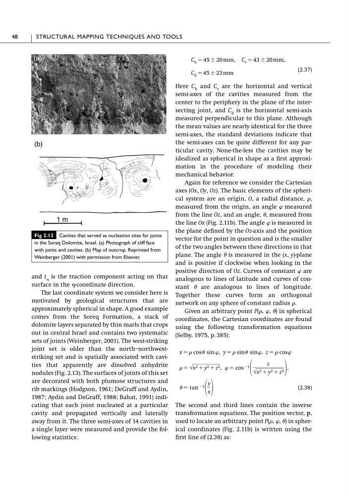
joint set is older than the north–northweststriking set and is spatially associated with cavities that apparently are dissolved anhydrite
nodules (Fig. 2.13). The surfaces of joints of this set
are decorated with both plumose structures and
rib markings (Hodgson, 1961; DeGraff and Aydin,
1987; Aydin and DeGraff, 1988; Bahat, 1991) indicating that each joint nucleated at a particular
cavity and propagated vertically and laterally
away from it. The three semi-axes of 14 cavities in
a single layer were measured and provide the following statistics:
(2.37)
Here C h and C v are the horizontal and vertical
semi-axes of the cavities measured from the
center to the periphery in the plane of the intersecting joint, and C d is the horizontal semi-axis
measured perpendicular to this plane. Although
the mean values are nearly identical for the three
semi-axes, the standard deviations indicate that
the semi-axes can be quite different for any particular cavity. None-the-less the cavities may be
idealized as spherical in shape as a first approximation in the procedure of modeling their
mechanical behavior.
Again for reference we consider the Cartesian
axes (Ox, Oy, Oz). The basic elements of the spherical system are an origin, O, a radial distance, �,
measured from the origin, an angle � measured
from the line Oz, and an angle, �, measured from
the line Ox (Fig. 2.11b). The angle � is measured in
the plane defined by the Oz-axis and the position
vector for the point in question and is the smaller
of the two angles between these directions in that
plane. The angle � is measured in the (x, y)-plane
and is positive if clockwise when looking in the
positive direction of Oz. Curves of constant � are
analogous to lines of latitude and curves of constant � are analogous to lines of longitude.
Together these curves form an orthogonal
network on any sphere of constant radius �.
Given an arbitrary point P(�, �, �) in spherical
coordinates, the Cartesian coordinates are found
using the following transformation equations
(Selby, 1975, p. 385):
(2.38)
The second and third lines contain the inverse
transformation equations. The position vector, p,
used to locate an arbitrary point P(�, �, �) in spherical coordinates (Fig. 2.11b) is written using the
first line of (2.38) as:
� � tan �1
y
x
� � √x 2 � y 2 � z 2 , � � cos �1
z
√x 2 � y 2 � z 2 ,
x � � cos� sin �, y � � sin� sin�, z � � cos�
C d � 45 � 23 mm
C h � 45 � 20 mm, C v � 43 � 20 mm,
48
STRUCTURAL MAPPING TECHNIQUES AND TOOLS
(a)
1 m
(b)
Fig 2.13 Cavities that served as nucleation sites for joints
in the Soreq Dolomite, Israel. (a) Photograph of cliff face
with joints and cavities. (b) Map of outcrop. Reprinted from
Weinberger (2001) with permission from Elsevier.
surface in the �-coordinate direction.
The last coordinate system we consider here is
motivated by geological structures that are
approximately spherical in shape. A good example
comes from the Soreq Formation, a stack of
dolomite layers separated by thin marls that crops
out in central Israel and contains two systematic
sets of joints (Weinberger, 2001). The west-striking
joint set is older than the north–northweststriking set and is spatially associated with cavities that apparently are dissolved anhydrite
nodules (Fig. 2.13). The surfaces of joints of this set
are decorated with both plumose structures and
rib markings (Hodgson, 1961; DeGraff and Aydin,
1987; Aydin and DeGraff, 1988; Bahat, 1991) indicating that each joint nucleated at a particular
cavity and propagated vertically and laterally
away from it. The three semi-axes of 14 cavities in
a single layer were measured and provide the following statistics:
(2.37)
Here C h and C v are the horizontal and vertical
semi-axes of the cavities measured from the
center to the periphery in the plane of the intersecting joint, and C d is the horizontal semi-axis
measured perpendicular to this plane. Although
the mean values are nearly identical for the three
semi-axes, the standard deviations indicate that
the semi-axes can be quite different for any particular cavity. None-the-less the cavities may be
idealized as spherical in shape as a first approximation in the procedure of modeling their
mechanical behavior.
Again for reference we consider the Cartesian
axes (Ox, Oy, Oz). The basic elements of the spherical system are an origin, O, a radial distance, �,
measured from the origin, an angle � measured
from the line Oz, and an angle, �, measured from
the line Ox (Fig. 2.11b). The angle � is measured in
the plane defined by the Oz-axis and the position
vector for the point in question and is the smaller
of the two angles between these directions in that
plane. The angle � is measured in the (x, y)-plane
and is positive if clockwise when looking in the
positive direction of Oz. Curves of constant � are
analogous to lines of latitude and curves of constant � are analogous to lines of longitude.
Together these curves form an orthogonal
network on any sphere of constant radius �.
Given an arbitrary point P(�, �, �) in spherical
coordinates, the Cartesian coordinates are found
using the following transformation equations
(Selby, 1975, p. 385):
(2.38)
The second and third lines contain the inverse
transformation equations. The position vector, p,
used to locate an arbitrary point P(�, �, �) in spherical coordinates (Fig. 2.11b) is written using the
first line of (2.38) as:
� � tan �1
y
x
� � √x 2 � y 2 � z 2 , � � cos �1
z
√x 2 � y 2 � z 2 ,
x � � cos� sin �, y � � sin� sin�, z � � cos�
C d � 45 � 23 mm
C h � 45 � 20 mm, C v � 43 � 20 mm,
48
STRUCTURAL MAPPING TECHNIQUES AND TOOLS
(a)
1 m
(b)
Fig 2.13 Cavities that served as nucleation sites for joints
in the Soreq Dolomite, Israel. (a) Photograph of cliff face
with joints and cavities. (b) Map of outcrop. Reprinted from
Weinberger (2001) with permission from Elsevier.