

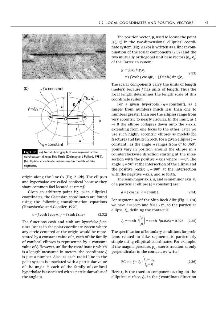
origin along the line Ox (Fig. 2.12b). The ellipses
and hyperbolae are called confocal because they
share common foci located at x ϭϮf.
Given an arbitrary point P(, ) in elliptical
coordinates, the Cartesian coordinates are found
using the following transformation equations
(Timoshenko and Goodier, 1970):
(2.32)
The functions cosh and sinh are hyperbolic functions. Just as in the polar coordinate system where
any circle centered at the origin would be represented by a constant value of r, each of the family
of confocal ellipses is represented by a constant
value of . However, unlike the coordinate r, which
is a length measured in meters, the coordinate
is just a number. Also, as each radial line in the
polar system is associated with a particular value
of the angle , each of the family of confocal
hyperbolae is associated with a particular value of
the angle .
x ϭ f cosh cos , y ϭ f sinh sin
The position vector, p, used to locate the point
P(, ) in the two-dimensional elliptical coordinate system (Fig. 2.12b) is written as a linear combination of the scalar components (2.32) and the
two mutually orthogonal unit base vectors (e x , e y )
of the Cartesian system:
(2.33)
The scalar components carry the units of length
(meters) because f has units of length. Thus the
focal length determines the length scale of this
coordinate system.
For a given hyperbola ( ϭ constant), as
ranges from numbers much less than one to
numbers greater than one the ellipses range from
very eccentric to nearly circular. In the limit, as
→ 0 the ellipse collapses down onto the x-axis,
extending from one focus to the other. Later we
use such highly eccentric ellipses as models for
fractures and faults in rock. For a given ellipse ( ϭ
constant), as the angle ranges from 0Њ to 360Њ,
points vary in position around the ellipse in a
counterclockwise direction starting at the intersection with the positive x-axis where ϭ 0Њ. The
angle ϭ 90Њ at the intersection of the ellipse and
the positive y-axis; ϭ 180Њ at the intersection
with the negative x-axis, and so forth.
The semi-major axis, a, and semi-minor axis, b,
of a particular ellipse ( ϭ constant) are:
(2.34)
For segment 16 of the Ship Rock dike (Fig. 2.12a)
we have a ϭ 68 m and b ϭ 1.7 m, so the particular
ellipse, O , defining the contact is:
(2.35)
The specification of boundary conditions for problems related to dike segments is particularly
simple using elliptical coordinates. For example,
if the magma pressure, p m , exerts traction, t, only
perpendicular to the contact, we write:
(2.36)
Here t is the traction component acting on the
elliptical surface, O , in the -coordinate direction
BC: on ϭ O Ά
t ϭ p m
t ϭ 0
O ϭ tanh Ϫ1
b
a ϭ tanh Ϫ1 (0.025) ϭ 0.025
a ϭ f cosh , b ϭ f sinh
ϭ ( f cosh cos )e x ϩ ( f sinh sin )e y
p ϭ p x e x ϩ p y e y
2.2 LOCAL COORDINATES AND POSITION VECTORS
47
(b)
x
y
f
P(j, h)
j = constant
h = constant
a
b
(a)
j = j O
p
O
Fig 2.12 (a) Aerial photograph of one segment of the
northeastern dike at Ship Rock (Delaney and Pollard, 1981).
(b) Elliptical coordinate system used in models of dike
segments.
and hyperbolae are called confocal because they
share common foci located at x ϭϮf.
Given an arbitrary point P(, ) in elliptical
coordinates, the Cartesian coordinates are found
using the following transformation equations
(Timoshenko and Goodier, 1970):
(2.32)
The functions cosh and sinh are hyperbolic functions. Just as in the polar coordinate system where
any circle centered at the origin would be represented by a constant value of r, each of the family
of confocal ellipses is represented by a constant
value of . However, unlike the coordinate r, which
is a length measured in meters, the coordinate
is just a number. Also, as each radial line in the
polar system is associated with a particular value
of the angle , each of the family of confocal
hyperbolae is associated with a particular value of
the angle .
x ϭ f cosh cos , y ϭ f sinh sin
The position vector, p, used to locate the point
P(, ) in the two-dimensional elliptical coordinate system (Fig. 2.12b) is written as a linear combination of the scalar components (2.32) and the
two mutually orthogonal unit base vectors (e x , e y )
of the Cartesian system:
(2.33)
The scalar components carry the units of length
(meters) because f has units of length. Thus the
focal length determines the length scale of this
coordinate system.
For a given hyperbola ( ϭ constant), as
ranges from numbers much less than one to
numbers greater than one the ellipses range from
very eccentric to nearly circular. In the limit, as
→ 0 the ellipse collapses down onto the x-axis,
extending from one focus to the other. Later we
use such highly eccentric ellipses as models for
fractures and faults in rock. For a given ellipse ( ϭ
constant), as the angle ranges from 0Њ to 360Њ,
points vary in position around the ellipse in a
counterclockwise direction starting at the intersection with the positive x-axis where ϭ 0Њ. The
angle ϭ 90Њ at the intersection of the ellipse and
the positive y-axis; ϭ 180Њ at the intersection
with the negative x-axis, and so forth.
The semi-major axis, a, and semi-minor axis, b,
of a particular ellipse ( ϭ constant) are:
(2.34)
For segment 16 of the Ship Rock dike (Fig. 2.12a)
we have a ϭ 68 m and b ϭ 1.7 m, so the particular
ellipse, O , defining the contact is:
(2.35)
The specification of boundary conditions for problems related to dike segments is particularly
simple using elliptical coordinates. For example,
if the magma pressure, p m , exerts traction, t, only
perpendicular to the contact, we write:
(2.36)
Here t is the traction component acting on the
elliptical surface, O , in the -coordinate direction
BC: on ϭ O Ά
t ϭ p m
t ϭ 0
O ϭ tanh Ϫ1
b
a ϭ tanh Ϫ1 (0.025) ϭ 0.025
a ϭ f cosh , b ϭ f sinh
ϭ ( f cosh cos )e x ϩ ( f sinh sin )e y
p ϭ p x e x ϩ p y e y
2.2 LOCAL COORDINATES AND POSITION VECTORS
47
(b)
x
y
f
P(j, h)
j = constant
h = constant
a
b
(a)
j = j O
p
O
Fig 2.12 (a) Aerial photograph of one segment of the
northeastern dike at Ship Rock (Delaney and Pollard, 1981).
(b) Elliptical coordinate system used in models of dike
segments.