

a table of directional cosines for rotation of position vector components using (2.23) as a template:
(2.27)
For example, one uses m zxЈ for the orthogonal projection of the z-component of the position vector
onto the xЈ-axis. Each new component of the position vector is composed of a linear combination of
the old components and the direction cosines in the
corresponding column of (2.27). Each old component of the position vector is composed of a linear
combination of the new components and the direction cosines in the corresponding row of (2.27).
Because the coordinates of an arbitrary point,
P(x, y, z), are equivalent to the components of the
position vector, p, for that point, the coordinates
can replace the components in (2.27) to form a
table of direction cosines for the rotational transformation of coordinates:
(2.28)
From this table we understand, for example, that
the direction cosine m yzЈ is used for the orthogonal
projection of the y-coordinate of P onto the zЈ-axis.
Each new coordinate of P is composed of a linear
combination of the old coordinates and the direction cosines in the corresponding column of
(2.28). The inverse transformation equations are
formed using the rows of this table. In summary
(2.23), (2.27), and (2.28) provide the equations for
both forward (old to new) and inverse (new to old)
rotational transformations for orthonormal base
vectors, for components of position vectors, and
for coordinates of points referred to rectangular
Cartesian coordinate systems.
Transformation equations that commonly are
employed in modeling structures include those
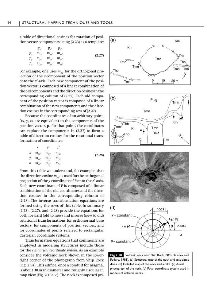
for the cylindrical coordinate system. As an example
consider the volcanic neck shown in the lowerright corner of the photograph from Ship Rock
(Fig. 2.5a). This edifice, once a conduit for magma,
is about 30 m in diameter and roughly circular in
map view (Fig. 2.10a, c). The neck is composed prixЈ
yЈ
zЈ
x m xxЈ m xyЈ m xzЈ
y m yxЈ m yyЈ m yzЈ
z m zxЈ m zyЈ m zzЈ
p xЈ
p yЈ
p zЈ
p x m xxЈ m xyЈ m xzЈ
p y m yxЈ m yyЈ m yzЈ
p z m zxЈ m zyЈ m zzЈ
44
STRUCTURAL MAPPING TECHNIQUES AND TOOLS
(d)
x
r = constant
u = constant
y
s
u
r
r = R
O
Km
Km
Tmn
Tmn
Tmn
Tmn
Km
Thb
Tmn
Thb
Thb
Thb
N
0
10
20 Meters
Thb
Thb
Km
Tmn
Tmn
Thb
Tmn
Dike
N
Km
Tmn
Tmn
Plug
0
2 Meters
Km
Km
Tmn
Tmn
Tmn
Tmn
Km
Thb
Tmn
Thb
Thb
Thb
N
0
10
20 m
Thb
Thb
Km
Tmn
Tmn
Thb
Tmn
Dike
N
Km
Tmn
Tmn
Plug
0
2 m
(a)
(b)
(c)
r cos u
P(r, u)
r sin u
Fig 2.10 Volcanic neck near Ship Rock, NM (Delaney and
Pollard, 1981). (a) Structural map of the neck and associated
dikes. (b) Detailed map of the neck and a dike. (c) Aerial
photograph of the neck. (d) Polar coordinate system used in
models of volcanic necks.
(2.27)
For example, one uses m zxЈ for the orthogonal projection of the z-component of the position vector
onto the xЈ-axis. Each new component of the position vector is composed of a linear combination of
the old components and the direction cosines in the
corresponding column of (2.27). Each old component of the position vector is composed of a linear
combination of the new components and the direction cosines in the corresponding row of (2.27).
Because the coordinates of an arbitrary point,
P(x, y, z), are equivalent to the components of the
position vector, p, for that point, the coordinates
can replace the components in (2.27) to form a
table of direction cosines for the rotational transformation of coordinates:
(2.28)
From this table we understand, for example, that
the direction cosine m yzЈ is used for the orthogonal
projection of the y-coordinate of P onto the zЈ-axis.
Each new coordinate of P is composed of a linear
combination of the old coordinates and the direction cosines in the corresponding column of
(2.28). The inverse transformation equations are
formed using the rows of this table. In summary
(2.23), (2.27), and (2.28) provide the equations for
both forward (old to new) and inverse (new to old)
rotational transformations for orthonormal base
vectors, for components of position vectors, and
for coordinates of points referred to rectangular
Cartesian coordinate systems.
Transformation equations that commonly are
employed in modeling structures include those
for the cylindrical coordinate system. As an example
consider the volcanic neck shown in the lowerright corner of the photograph from Ship Rock
(Fig. 2.5a). This edifice, once a conduit for magma,
is about 30 m in diameter and roughly circular in
map view (Fig. 2.10a, c). The neck is composed prixЈ
yЈ
zЈ
x m xxЈ m xyЈ m xzЈ
y m yxЈ m yyЈ m yzЈ
z m zxЈ m zyЈ m zzЈ
p xЈ
p yЈ
p zЈ
p x m xxЈ m xyЈ m xzЈ
p y m yxЈ m yyЈ m yzЈ
p z m zxЈ m zyЈ m zzЈ
44
STRUCTURAL MAPPING TECHNIQUES AND TOOLS
(d)
x
r = constant
u = constant
y
s
u
r
r = R
O
Km
Km
Tmn
Tmn
Tmn
Tmn
Km
Thb
Tmn
Thb
Thb
Thb
N
0
10
20 Meters
Thb
Thb
Km
Tmn
Tmn
Thb
Tmn
Dike
N
Km
Tmn
Tmn
Plug
0
2 Meters
Km
Km
Tmn
Tmn
Tmn
Tmn
Km
Thb
Tmn
Thb
Thb
Thb
N
0
10
20 m
Thb
Thb
Km
Tmn
Tmn
Thb
Tmn
Dike
N
Km
Tmn
Tmn
Plug
0
2 m
(a)
(b)
(c)
r cos u
P(r, u)
r sin u
Fig 2.10 Volcanic neck near Ship Rock, NM (Delaney and
Pollard, 1981). (a) Structural map of the neck and associated
dikes. (b) Detailed map of the neck and a dike. (c) Aerial
photograph of the neck. (d) Polar coordinate system used in
models of volcanic necks.