

(2.19)
Because the scalar product is written with a dot
between the two vectors, it is referred to as the dot
product. Here is the smaller of the two angles
between the lines directed parallel to v and w
measured in the plane defined by the two vectors
(Fig. 2.9b), so the product |v|cos is the orthogonal projection of v onto the line parallel to w. In
other words |v|cos is the component of v in the
direction of w. Therefore, the scalar product may
be interpreted geometrically as the product of the
component of v along w and the magnitude of w.
Alternatively, the scalar product may be interpreted as the product of the component of w
along v and the magnitude of v.
Two important relationships among the
vectors defining a basis are expressed conveniently using the scalar product (2.19):
(2.20)
These relations are interpreted by recalling that
orthonormal basis vectors are of unit magnitude
and they are mutually orthogonal to one another.
For the rotational transformation we want, for
example, to project e x , e y , and e z onto the line parallel to e xЈ (Fig. 2.9a). These projections are accomplished using the scalar product (2.19) and
recalling that the base vectors are unit vectors:
(2.21)
Analogous procedures are used to project e x , e y ,
and e z onto lines parallel to e yЈ and e zЈ and these
operations define nine direction cosines that relate
the old basis to the new basis:
(2.22)
Here the double subscripts on the direction
cosines refer to the reference (old) axis and the
transformed (new) axis, respectively.
m zzЈ ϭ cos (z, zЈ)
m zxЈ ϭ cos (z, xЈ), m zyЈ ϭ cos (z, yЈ),
m yzЈ ϭ cos (y, zЈ)
m yxЈ ϭ cos (y, xЈ), m yyЈ ϭ cos (y, yЈ),
m xzЈ ϭ cos (x, zЈ)
m xxЈ ϭ cos (x, xЈ), m xyЈ ϭ cos (x, yЈ),
e z · e xЈ ϭ |e z ||e xЈ |cos (z, xЈ) ϭ cos (z, xЈ) ϭ m zxЈ
e y · e xЈ ϭ |e y ||e xЈ | cos (y, xЈ) ϭ cos (y, xЈ) ϭ m yxЈ
e x · e xЈ ϭ |e x ||e xЈ |cos (x, xЈ) ϭ cos (x, xЈ) ϭ m xxЈ
e x · e y ϭ e y · e z ϭ e z · e x ϭ 0
e x · e x ϭ e y · e y ϭ e z · e z ϭ 1
ϭ v x w x ϩ v y w y ϩ v z w z
v · w ϭ |v||w| cos , for 0 Յ Յ
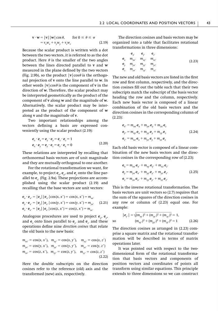
The direction cosines and basis vectors may be
organized into a table that facilitates rotational
transformations in three dimensions:
(2.23)
The new and old basis vectors are listed in the first
row and first column, respectively, and the direction cosines fill out the table such that their two
subscripts match the subscript of the basis vector
heading the row and the column, respectively.
Each new basis vector is composed of a linear
combination of the old basis vectors and the
direction cosines in the corresponding column of
(2.23):
(2.24)
Each old basis vector is composed of a linear combination of the new basis vectors and the direction cosines in the corresponding row of (2.23):
(2.25)
This is the inverse rotational transformation. The
basis vectors are unit vectors so (2.7) requires that
the sum of the squares of the direction cosines in
any row or column of (2.23) equal one. For
example:
so
(2.26)
The direction cosines as arranged in (2.23) comprise a square matrix and the rotational transformation will be described in terms of matrix
operations later.
It was pointed out with respect to the twodimensional form of the rotational transformation that basis vectors and components of
position vectors and coordinates of points all
transform using similar equations. This principle
extends to three dimensions so we can construct
(m xyЈ ) 2 ϩ (m yyЈ ) 2 ϩ (m zyЈ ) 2 ϭ 1
|e yЈ | ϭ √ (m xyЈ ) 2 ϩ (m yyЈ ) 2 ϩ (m zyЈ ) 2 ϭ 1,
e z ϭ m zxЈ e xЈ ϩ m zyЈ e yЈ ϩ m zzЈ e zЈ
e y ϭ m yxЈ e xЈ ϩ m yyЈ e yЈ ϩ m yzЈ e zЈ
e x ϭ m xxЈ e xЈ ϩ m xyЈ e yЈ ϩ m xzЈ e zЈ
e zЈ ϭ m xzЈ e x ϩ m yzЈ e y ϩ m zzЈ e z
e yЈ ϭ m xyЈ e x ϩ m yyЈ e y ϩ m zyЈ e z
e xЈ ϭ m xxЈ e x ϩ m yxЈ e y ϩ m zxЈ e z
e xЈ
e yЈ
e zЈ
e x m xxЈ m xyЈ m xzЈ
e y m yxЈ m yyЈ m yzЈ
e z m zxЈ m zyЈ m zzЈ
2.2 LOCAL COORDINATES AND POSITION VECTORS
43
Because the scalar product is written with a dot
between the two vectors, it is referred to as the dot
product. Here is the smaller of the two angles
between the lines directed parallel to v and w
measured in the plane defined by the two vectors
(Fig. 2.9b), so the product |v|cos is the orthogonal projection of v onto the line parallel to w. In
other words |v|cos is the component of v in the
direction of w. Therefore, the scalar product may
be interpreted geometrically as the product of the
component of v along w and the magnitude of w.
Alternatively, the scalar product may be interpreted as the product of the component of w
along v and the magnitude of v.
Two important relationships among the
vectors defining a basis are expressed conveniently using the scalar product (2.19):
(2.20)
These relations are interpreted by recalling that
orthonormal basis vectors are of unit magnitude
and they are mutually orthogonal to one another.
For the rotational transformation we want, for
example, to project e x , e y , and e z onto the line parallel to e xЈ (Fig. 2.9a). These projections are accomplished using the scalar product (2.19) and
recalling that the base vectors are unit vectors:
(2.21)
Analogous procedures are used to project e x , e y ,
and e z onto lines parallel to e yЈ and e zЈ and these
operations define nine direction cosines that relate
the old basis to the new basis:
(2.22)
Here the double subscripts on the direction
cosines refer to the reference (old) axis and the
transformed (new) axis, respectively.
m zzЈ ϭ cos (z, zЈ)
m zxЈ ϭ cos (z, xЈ), m zyЈ ϭ cos (z, yЈ),
m yzЈ ϭ cos (y, zЈ)
m yxЈ ϭ cos (y, xЈ), m yyЈ ϭ cos (y, yЈ),
m xzЈ ϭ cos (x, zЈ)
m xxЈ ϭ cos (x, xЈ), m xyЈ ϭ cos (x, yЈ),
e z · e xЈ ϭ |e z ||e xЈ |cos (z, xЈ) ϭ cos (z, xЈ) ϭ m zxЈ
e y · e xЈ ϭ |e y ||e xЈ | cos (y, xЈ) ϭ cos (y, xЈ) ϭ m yxЈ
e x · e xЈ ϭ |e x ||e xЈ |cos (x, xЈ) ϭ cos (x, xЈ) ϭ m xxЈ
e x · e y ϭ e y · e z ϭ e z · e x ϭ 0
e x · e x ϭ e y · e y ϭ e z · e z ϭ 1
ϭ v x w x ϩ v y w y ϩ v z w z
v · w ϭ |v||w| cos , for 0 Յ Յ
The direction cosines and basis vectors may be
organized into a table that facilitates rotational
transformations in three dimensions:
(2.23)
The new and old basis vectors are listed in the first
row and first column, respectively, and the direction cosines fill out the table such that their two
subscripts match the subscript of the basis vector
heading the row and the column, respectively.
Each new basis vector is composed of a linear
combination of the old basis vectors and the
direction cosines in the corresponding column of
(2.23):
(2.24)
Each old basis vector is composed of a linear combination of the new basis vectors and the direction cosines in the corresponding row of (2.23):
(2.25)
This is the inverse rotational transformation. The
basis vectors are unit vectors so (2.7) requires that
the sum of the squares of the direction cosines in
any row or column of (2.23) equal one. For
example:
so
(2.26)
The direction cosines as arranged in (2.23) comprise a square matrix and the rotational transformation will be described in terms of matrix
operations later.
It was pointed out with respect to the twodimensional form of the rotational transformation that basis vectors and components of
position vectors and coordinates of points all
transform using similar equations. This principle
extends to three dimensions so we can construct
(m xyЈ ) 2 ϩ (m yyЈ ) 2 ϩ (m zyЈ ) 2 ϭ 1
|e yЈ | ϭ √ (m xyЈ ) 2 ϩ (m yyЈ ) 2 ϩ (m zyЈ ) 2 ϭ 1,
e z ϭ m zxЈ e xЈ ϩ m zyЈ e yЈ ϩ m zzЈ e zЈ
e y ϭ m yxЈ e xЈ ϩ m yyЈ e yЈ ϩ m yzЈ e zЈ
e x ϭ m xxЈ e xЈ ϩ m xyЈ e yЈ ϩ m xzЈ e zЈ
e zЈ ϭ m xzЈ e x ϩ m yzЈ e y ϩ m zzЈ e z
e yЈ ϭ m xyЈ e x ϩ m yyЈ e y ϩ m zyЈ e z
e xЈ ϭ m xxЈ e x ϩ m yxЈ e y ϩ m zxЈ e z
e xЈ
e yЈ
e zЈ
e x m xxЈ m xyЈ m xzЈ
e y m yxЈ m yyЈ m yzЈ
e z m zxЈ m zyЈ m zzЈ
2.2 LOCAL COORDINATES AND POSITION VECTORS
43