

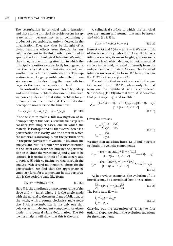
The perturbation in principal axis orientation
and those in the principal viscosities occur in separate terms, because any term containing a
product of a perturbing quantity is deleted in the
linearization. They may thus be thought of as
giving separate effects even though for any
volume element in the fluid both are required to
specify the local rheological behavior. We might
thus imagine one limiting situation in which the
principal viscosities were perfectly homogeneous
but the principal axis orientation varied, and
another in which the opposite was true. This separation is no longer possible when the dimensionless quantities describing them are both too
large for the linearized equations to hold.
In contrast to the many examples of boundary
and initial value problems discussed in this text,
we now consider an initial value problem for an
unbounded volume of material. The initial value
description now refers to the functions:
(11.112)
If one wishes to make a full investigation of inhomogeneity of this sort, a sensible first step is to
consider two simpler cases, one in which the
material is isotropic and all that is considered is a
perturbation in viscosity, and the other in which
the material is anisotropic, but the perturbations
in the principal viscosities vanish. To illustrate the
analysis and results further, we restrict attention
to the latter case, described only by the perturbation in . Since the variations ␦ n and ␦ s are to be
ignored, it is useful to think of them as zero and
to replace with m. Having worked through the
analysis with several mathematical forms for the
perturbation, we find that the appropriate elementary form for a component in this perturbation is the periodic band-like form:
(11.113)
Here ⌰ is the amplitude or maximum value of the
slope and
, where  is the angle made
with the normal to the mean plane of foliation, or
the y-axis, with a counterclockwise angle negative. Such a perturbation is the only one that
behaves as an independent component, or eigenmode, in a general plane deformation. The following analysis will show that this is the case.
ϭ tan 
(x, y) ϭ Ϫ⌰ sin (x Ϫ y)
m
ϭ (x, y), ␦ n ϭ ␦ n (x, y), ␦ s ϭ ␦ s (x, y)
A cylindrical surface to which the principal
axes are tangent and normal that may be associated with (11.113) is:
(11.114)
Here ⌰ ϭA and
We may think
of the trace of a cylindrical surface (11.114) as a
foliation surface; its mean height, above some
reference level, which defines, in part, a material
surface in the fluid, is treated differently from the
independent coordinate y. An example of a set of
foliation surfaces of the form (11.114) is shown in
Fig. 11.22 for the case  ϭϪ45Њ.
The solution that we seek starts with the particular solution to (11.111), where only the first
term on the right-hand side is considered.
Substituting (11.113) into that term, it is then clear
that ϳ sin(x Ϫ y), and we obtain:
(11.115)
Given the stresses:
(11.116)
We may then substitute into (11.110) and integrate
to obtain the velocity components:
(11.117)
As in previous examples, the evolution of the
interface may be determined from the relation:
(11.118)
The basic-state flow is:
(11.119)
Carrying out the expansion of (11.118) to first
order in slope, we obtain the evolution equations
for the component:
v y ϭ ϪD xx y
v x ϭ D xx x ϩ 2D xy y
Ѩ
Ѩt
ϭ v y (x, ) Ϫ v x (x, )
Ѩ
Ѩx
v ~ y ϭ
Ϫ4(m Ϫ 1) [2D xy ϩ (1 Ϫ
2 )D xx ]
[1 ϩ 2(2m Ϫ 1)
2 ϩ
4 ]
A cos (x Ϫ y)
v ~ x ϭ
Ϫ4(m Ϫ 1) [2D xy ϩ (1 Ϫ
2
)D xx ]
[1 ϩ 2(2m Ϫ 1)
2 ϩ
4 ]
A cos (x Ϫ y)
s
~ xy ϭ Ϫ
Ѩ 2
ѨyѨx
s
~ xx ϭ
1
2
Ѩ 2
Ѩy 2 Ϫ
Ѩ 2
Ѩx 2
ϭ Ϫ
(1ր 2 )(4m Ϫ 1)[(Ϫ 2 ϩ 1)s xy 2 s xx ]⌰ sin (x Ϫ y)
[1 ϩ (2m Ϫ 1) 2 ϩ 4 ]
y,
Ѩ րѨx ϭ tan Х .
(x, y) ϭ y ϩ A cos (x Ϫ y)
452
RHEOLOGICAL BEHAVIOR
and those in the principal viscosities occur in separate terms, because any term containing a
product of a perturbing quantity is deleted in the
linearization. They may thus be thought of as
giving separate effects even though for any
volume element in the fluid both are required to
specify the local rheological behavior. We might
thus imagine one limiting situation in which the
principal viscosities were perfectly homogeneous
but the principal axis orientation varied, and
another in which the opposite was true. This separation is no longer possible when the dimensionless quantities describing them are both too
large for the linearized equations to hold.
In contrast to the many examples of boundary
and initial value problems discussed in this text,
we now consider an initial value problem for an
unbounded volume of material. The initial value
description now refers to the functions:
(11.112)
If one wishes to make a full investigation of inhomogeneity of this sort, a sensible first step is to
consider two simpler cases, one in which the
material is isotropic and all that is considered is a
perturbation in viscosity, and the other in which
the material is anisotropic, but the perturbations
in the principal viscosities vanish. To illustrate the
analysis and results further, we restrict attention
to the latter case, described only by the perturbation in . Since the variations ␦ n and ␦ s are to be
ignored, it is useful to think of them as zero and
to replace with m. Having worked through the
analysis with several mathematical forms for the
perturbation, we find that the appropriate elementary form for a component in this perturbation is the periodic band-like form:
(11.113)
Here ⌰ is the amplitude or maximum value of the
slope and
, where  is the angle made
with the normal to the mean plane of foliation, or
the y-axis, with a counterclockwise angle negative. Such a perturbation is the only one that
behaves as an independent component, or eigenmode, in a general plane deformation. The following analysis will show that this is the case.
ϭ tan 
(x, y) ϭ Ϫ⌰ sin (x Ϫ y)
m
ϭ (x, y), ␦ n ϭ ␦ n (x, y), ␦ s ϭ ␦ s (x, y)
A cylindrical surface to which the principal
axes are tangent and normal that may be associated with (11.113) is:
(11.114)
Here ⌰ ϭA and
We may think
of the trace of a cylindrical surface (11.114) as a
foliation surface; its mean height, above some
reference level, which defines, in part, a material
surface in the fluid, is treated differently from the
independent coordinate y. An example of a set of
foliation surfaces of the form (11.114) is shown in
Fig. 11.22 for the case  ϭϪ45Њ.
The solution that we seek starts with the particular solution to (11.111), where only the first
term on the right-hand side is considered.
Substituting (11.113) into that term, it is then clear
that ϳ sin(x Ϫ y), and we obtain:
(11.115)
Given the stresses:
(11.116)
We may then substitute into (11.110) and integrate
to obtain the velocity components:
(11.117)
As in previous examples, the evolution of the
interface may be determined from the relation:
(11.118)
The basic-state flow is:
(11.119)
Carrying out the expansion of (11.118) to first
order in slope, we obtain the evolution equations
for the component:
v y ϭ ϪD xx y
v x ϭ D xx x ϩ 2D xy y
Ѩ
Ѩt
ϭ v y (x, ) Ϫ v x (x, )
Ѩ
Ѩx
v ~ y ϭ
Ϫ4(m Ϫ 1) [2D xy ϩ (1 Ϫ
2 )D xx ]
[1 ϩ 2(2m Ϫ 1)
2 ϩ
4 ]
A cos (x Ϫ y)
v ~ x ϭ
Ϫ4(m Ϫ 1) [2D xy ϩ (1 Ϫ
2
)D xx ]
[1 ϩ 2(2m Ϫ 1)
2 ϩ
4 ]
A cos (x Ϫ y)
s
~ xy ϭ Ϫ
Ѩ 2
ѨyѨx
s
~ xx ϭ
1
2
Ѩ 2
Ѩy 2 Ϫ
Ѩ 2
Ѩx 2
ϭ Ϫ
(1ր 2 )(4m Ϫ 1)[(Ϫ 2 ϩ 1)s xy 2 s xx ]⌰ sin (x Ϫ y)
[1 ϩ (2m Ϫ 1) 2 ϩ 4 ]
y,
Ѩ րѨx ϭ tan Х .
(x, y) ϭ y ϩ A cos (x Ϫ y)
452
RHEOLOGICAL BEHAVIOR