

metry of behaviors for high-viscosity inclusions in
low-viscosity material versus low-viscosity inclusions in high-viscosity material, an asymmetry not
contained in the Voight and Reuss estimates.
Consider again a composite composed of two
isotropic viscous components. Paul models a composite material in terms of a simple representative
volume element (RVE) of it in the form of a unit
cube. For definiteness, he also considered specific
simple, if somewhat idealized, configurations of
the components within this RVE. The component
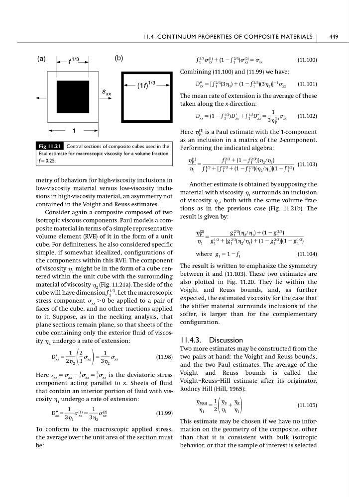
of viscosity 1 might be in the form of a cube centered within the unit cube with the surrounding
material of viscosity 2 (Fig. 11.21a). The side of the
cube will have dimension
. Let the macroscopic
stress component xx Ͼ 0 be applied to a pair of
faces of the cube, and no other tractions applied
to it. Suppose, as in the necking analysis, that
plane sections remain plane, so that sheets of the
cube containing only the exterior fluid of viscosity 2 undergo a rate of extension:
(11.98)
Here
is the deviatoric stress
component acting parallel to x. Sheets of fluid
that contain an interior portion of fluid with viscosity 1 undergo a rate of extension:
(11.99)
To conform to the macroscopic applied stress,
the average over the unit area of the section must
be:
D xx Љ ϭ
1
3 1
(1)
xx ϭ
1
3 2
(2)
xx
s xx ϭ xx Ϫ
1
3 xx ϭ
2
3 xx
DЈ xx ϭ
1
2 2
2
3
xx ϭ
1
3 2
xx
f
1ր3
1
(11.100)
Combining (11.100) and (11.99) we have:
(11.101)
The mean rate of extension is the average of these
taken along the x-direction:
(11.102)
Here
is a Paul estimate with the 1-component
as an inclusion in a matrix of the 2-component.
Performing the indicated algebra:
(11.103)
Another estimate is obtained by supposing the
material with viscosity 1 surrounds an inclusion
of viscosity 2 , both with the same volume fractions as in the previous case (Fig. 11.21b). The
result is given by:
(11.104)
The result is written to emphasize the symmetry
between it and (11.103). These two estimates are
also plotted in Fig. 11.20. They lie within the
Voight and Reuss bounds, and, as further
expected, the estimated viscosity for the case that
the stiffer material surrounds inclusions of the
softer, is larger than for the complementary
configuration.
11.4.3. Discussion
Two more estimates may be constructed from the
two pairs at hand: the Voight and Reuss bounds,
and the two Paul estimates. The average of the
Voight and Reuss bounds is called the
Voight–Reuss–Hill estimate after its originator,
Rodney Hill (Hill, 1965):
(11.105)
This estimate may be chosen if we have no information on the geometry of the composite, other
than that it is consistent with bulk isotropic
behavior, or that the sample of interest is selected
VRH
1
ϭ
1
2
V
1
ϩ
R
1
where g 1 ϭ 1 Ϫ f 1
(2)
P
1
ϭ
g 2ր3
1 ( 2 ր 1 ) ϩ (1 Ϫ g 2ր3
1 )
g 1ր3
1 ϩ [g 2ր3
1 ( 2 ր 1 ) ϩ (1 Ϫ g 2ր3
1 )](1 Ϫ g 1ր3
1 )
(1)
P
1
ϭ
f 2ր3
1 ϩ (1 Ϫ f 2ր3
1 )( 2 ր 1 )
f 1ր3
1 ϩ [ f 2ր3
1 ϩ (1 Ϫ f 2ր3
1 )( 2 ր 1 )](1 Ϫ f 1ր3
1 )
(1)
P
D xx ϭ (1 Ϫ f 1ր3
1 ) DЈ xx ϩ f 1ր3
1 DЉ xx ϭ
1
3
(1)
P
xx
DЉ xx ϭ [ f 2ր3
1 (3 1 ) ϩ (1 Ϫ f 2ր3
1 )(3 2 )] Ϫ1 xx
f 2ր3
1 (1)
xx ϩ (1 Ϫ f 2ր3
1 ) (2)
xx ϭ xx
11.4 CONTINUUM PROPERTIES OF COMPOSITE MATERIALS
449
Fig 11.21 Central sections of composite cubes used in the
Paul estimate for macroscopic viscosity for a volume fraction
fϭ 0.25.
f
1/3
s xx
1
(1f)
1/3
(a)
(b)
low-viscosity material versus low-viscosity inclusions in high-viscosity material, an asymmetry not
contained in the Voight and Reuss estimates.
Consider again a composite composed of two
isotropic viscous components. Paul models a composite material in terms of a simple representative
volume element (RVE) of it in the form of a unit
cube. For definiteness, he also considered specific
simple, if somewhat idealized, configurations of
the components within this RVE. The component
of viscosity 1 might be in the form of a cube centered within the unit cube with the surrounding
material of viscosity 2 (Fig. 11.21a). The side of the
cube will have dimension
. Let the macroscopic
stress component xx Ͼ 0 be applied to a pair of
faces of the cube, and no other tractions applied
to it. Suppose, as in the necking analysis, that
plane sections remain plane, so that sheets of the
cube containing only the exterior fluid of viscosity 2 undergo a rate of extension:
(11.98)
Here
is the deviatoric stress
component acting parallel to x. Sheets of fluid
that contain an interior portion of fluid with viscosity 1 undergo a rate of extension:
(11.99)
To conform to the macroscopic applied stress,
the average over the unit area of the section must
be:
D xx Љ ϭ
1
3 1
(1)
xx ϭ
1
3 2
(2)
xx
s xx ϭ xx Ϫ
1
3 xx ϭ
2
3 xx
DЈ xx ϭ
1
2 2
2
3
xx ϭ
1
3 2
xx
f
1ր3
1
(11.100)
Combining (11.100) and (11.99) we have:
(11.101)
The mean rate of extension is the average of these
taken along the x-direction:
(11.102)
Here
is a Paul estimate with the 1-component
as an inclusion in a matrix of the 2-component.
Performing the indicated algebra:
(11.103)
Another estimate is obtained by supposing the
material with viscosity 1 surrounds an inclusion
of viscosity 2 , both with the same volume fractions as in the previous case (Fig. 11.21b). The
result is given by:
(11.104)
The result is written to emphasize the symmetry
between it and (11.103). These two estimates are
also plotted in Fig. 11.20. They lie within the
Voight and Reuss bounds, and, as further
expected, the estimated viscosity for the case that
the stiffer material surrounds inclusions of the
softer, is larger than for the complementary
configuration.
11.4.3. Discussion
Two more estimates may be constructed from the
two pairs at hand: the Voight and Reuss bounds,
and the two Paul estimates. The average of the
Voight and Reuss bounds is called the
Voight–Reuss–Hill estimate after its originator,
Rodney Hill (Hill, 1965):
(11.105)
This estimate may be chosen if we have no information on the geometry of the composite, other
than that it is consistent with bulk isotropic
behavior, or that the sample of interest is selected
VRH
1
ϭ
1
2
V
1
ϩ
R
1
where g 1 ϭ 1 Ϫ f 1
(2)
P
1
ϭ
g 2ր3
1 ( 2 ր 1 ) ϩ (1 Ϫ g 2ր3
1 )
g 1ր3
1 ϩ [g 2ր3
1 ( 2 ր 1 ) ϩ (1 Ϫ g 2ր3
1 )](1 Ϫ g 1ր3
1 )
(1)
P
1
ϭ
f 2ր3
1 ϩ (1 Ϫ f 2ր3
1 )( 2 ր 1 )
f 1ր3
1 ϩ [ f 2ր3
1 ϩ (1 Ϫ f 2ր3
1 )( 2 ր 1 )](1 Ϫ f 1ր3
1 )
(1)
P
D xx ϭ (1 Ϫ f 1ր3
1 ) DЈ xx ϩ f 1ր3
1 DЉ xx ϭ
1
3
(1)
P
xx
DЉ xx ϭ [ f 2ր3
1 (3 1 ) ϩ (1 Ϫ f 2ր3
1 )(3 2 )] Ϫ1 xx
f 2ր3
1 (1)
xx ϩ (1 Ϫ f 2ր3
1 ) (2)
xx ϭ xx
11.4 CONTINUUM PROPERTIES OF COMPOSITE MATERIALS
449
Fig 11.21 Central sections of composite cubes used in the
Paul estimate for macroscopic viscosity for a volume fraction
fϭ 0.25.
f
1/3
s xx
1
(1f)
1/3
(a)
(b)