

Thus, in the present formulation, such a stress distribution would give no dilatation, even though
the gradient in mean stress is not zero. The relation (11.81) is obtained by substituting the stress
components into the constitutive relations for an
incompressible viscous fluid, and these in turn into
the equation of compatibility. Repeating this
here, but with the present constitutive relations,
we obtain:
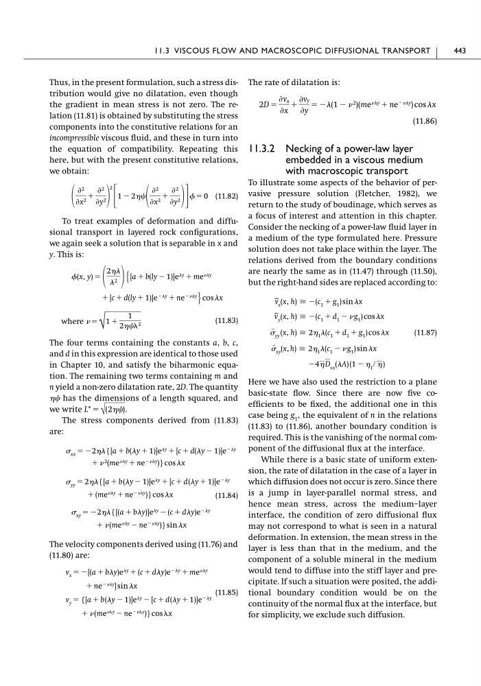
(11.82)
To treat examples of deformation and diffusional transport in layered rock configurations,
we again seek a solution that is separable in x and
y. This is:
(11.83)
The four terms containing the constants a, b, c,
and d in this expression are identical to those used
in Chapter 10, and satisfy the biharmonic equation. The remaining two terms containing m and
n yield a non-zero dilatation rate, 2D. The quantity
has the dimensions of a length squared, and
we write
The stress components derived from (11.83)
are:
(11.84)
The velocity components derived using (11.76) and
(11.80) are:
(11.85)
ϩ (me y Ϫ ne Ϫy )} cos x
v y ϭ {[a ϩ b(y Ϫ 1)]e y Ϫ [c ϩ d(y ϩ 1)]e Ϫy
ϩ ne Ϫy ] sin x
v x ϭ Ϫ[(a ϩ by)e y ϩ (c ϩ dy)e Ϫy ϩ me y
ϩ (me y Ϫ ne Ϫy )} sin x
xy ϭ Ϫ2{[(a ϩ by)]e y Ϫ (c ϩ dy)e Ϫy
ϩ (me y ϩ ne Ϫy )} cos x
yy ϭ 2{[a ϩ b(y Ϫ 1)]e y ϩ [c ϩ d(y ϩ 1)]e Ϫy
ϩ 2 (me y ϩ ne Ϫy )} cos x
xx ϭ Ϫ2{[a ϩ b(y ϩ 1)]e y ϩ [c ϩ d(y Ϫ 1)]e Ϫy
L* ϭ √ (2).
where ϭ
√
1 ϩ
1
2 2
ϩ [c ϩ d(ly ϩ 1)]e Ϫy ϩ ne Ϫy · cos x
(x, y) ϭ
2
2 Ά [a ϩ b(ly Ϫ 1)]e y ϩ me y
Ѩ 2
Ѩx 2 ϩ
Ѩ 2
Ѩy 2
2
΄ 1 Ϫ 2
Ѩ 2
Ѩx 2 ϩ
Ѩ 2
Ѩy 2 ΅ ϭ 0
The rate of dilatation is:
(11.86)
11.3.2 Necking of a power-law layer
embedded in a viscous medium
with macroscopic transport
To illustrate some aspects of the behavior of pervasive pressure solution (Fletcher, 1982), we
return to the study of boudinage, which serves as
a focus of interest and attention in this chapter.
Consider the necking of a power-law fluid layer in
a medium of the type formulated here. Pressure
solution does not take place within the layer. The
relations derived from the boundary conditions
are nearly the same as in (11.47) through (11.50),
but the right-hand sides are replaced according to:
(11.87)
Here we have also used the restriction to a plane
basic-state flow. Since there are now five coefficients to be fixed, the additional one in this
case being g 1 , the equivalent of n in the relations
(11.83) to (11.86), another boundary condition is
required. This is the vanishing of the normal component of the diffusional flux at the interface.
While there is a basic state of uniform extension, the rate of dilatation in the case of a layer in
which diffusion does not occur is zero. Since there
is a jump in layer-parallel normal stress, and
hence mean stress, across the medium–layer
interface, the condition of zero diffusional flux
may not correspond to what is seen in a natural
deformation. In extension, the mean stress in the
layer is less than that in the medium, and the
component of a soluble mineral in the medium
would tend to diffuse into the stiff layer and precipitate. If such a situation were posited, the additional boundary condition would be on the
continuity of the normal flux at the interface, but
for simplicity, we exclude such diffusion.
Ϫ4 D xx (A) (1 Ϫ 1 ր )
~
xy (x, h) Х 2 1 (c 1 Ϫ g 1 ) sin x
~
yy (x, h) Х 2 1 (c 1 ϩ d 1 ϩ g 1 ) cos x
v
~ y (x, h) Х Ϫ(c 1 ϩ d 1 Ϫ g 1 ) cos x
~ vs x (x, h) Х Ϫ(c 1 ϩ g 1 ) sin x
2D ϭ
Ѩv x
Ѩx
ϩ
Ѩvy
Ѩy
ϭ Ϫ(1 Ϫ 2 )(me y ϩ ne Ϫy ) cos x
11.3 VISCOUS FLOW AND MACROSCOPIC DIFFUSIONAL TRANSPORT
443
the gradient in mean stress is not zero. The relation (11.81) is obtained by substituting the stress
components into the constitutive relations for an
incompressible viscous fluid, and these in turn into
the equation of compatibility. Repeating this
here, but with the present constitutive relations,
we obtain:
(11.82)
To treat examples of deformation and diffusional transport in layered rock configurations,
we again seek a solution that is separable in x and
y. This is:
(11.83)
The four terms containing the constants a, b, c,
and d in this expression are identical to those used
in Chapter 10, and satisfy the biharmonic equation. The remaining two terms containing m and
n yield a non-zero dilatation rate, 2D. The quantity
has the dimensions of a length squared, and
we write
The stress components derived from (11.83)
are:
(11.84)
The velocity components derived using (11.76) and
(11.80) are:
(11.85)
ϩ (me y Ϫ ne Ϫy )} cos x
v y ϭ {[a ϩ b(y Ϫ 1)]e y Ϫ [c ϩ d(y ϩ 1)]e Ϫy
ϩ ne Ϫy ] sin x
v x ϭ Ϫ[(a ϩ by)e y ϩ (c ϩ dy)e Ϫy ϩ me y
ϩ (me y Ϫ ne Ϫy )} sin x
xy ϭ Ϫ2{[(a ϩ by)]e y Ϫ (c ϩ dy)e Ϫy
ϩ (me y ϩ ne Ϫy )} cos x
yy ϭ 2{[a ϩ b(y Ϫ 1)]e y ϩ [c ϩ d(y ϩ 1)]e Ϫy
ϩ 2 (me y ϩ ne Ϫy )} cos x
xx ϭ Ϫ2{[a ϩ b(y ϩ 1)]e y ϩ [c ϩ d(y Ϫ 1)]e Ϫy
L* ϭ √ (2).
where ϭ
√
1 ϩ
1
2 2
ϩ [c ϩ d(ly ϩ 1)]e Ϫy ϩ ne Ϫy · cos x
(x, y) ϭ
2
2 Ά [a ϩ b(ly Ϫ 1)]e y ϩ me y
Ѩ 2
Ѩx 2 ϩ
Ѩ 2
Ѩy 2
2
΄ 1 Ϫ 2
Ѩ 2
Ѩx 2 ϩ
Ѩ 2
Ѩy 2 ΅ ϭ 0
The rate of dilatation is:
(11.86)
11.3.2 Necking of a power-law layer
embedded in a viscous medium
with macroscopic transport
To illustrate some aspects of the behavior of pervasive pressure solution (Fletcher, 1982), we
return to the study of boudinage, which serves as
a focus of interest and attention in this chapter.
Consider the necking of a power-law fluid layer in
a medium of the type formulated here. Pressure
solution does not take place within the layer. The
relations derived from the boundary conditions
are nearly the same as in (11.47) through (11.50),
but the right-hand sides are replaced according to:
(11.87)
Here we have also used the restriction to a plane
basic-state flow. Since there are now five coefficients to be fixed, the additional one in this
case being g 1 , the equivalent of n in the relations
(11.83) to (11.86), another boundary condition is
required. This is the vanishing of the normal component of the diffusional flux at the interface.
While there is a basic state of uniform extension, the rate of dilatation in the case of a layer in
which diffusion does not occur is zero. Since there
is a jump in layer-parallel normal stress, and
hence mean stress, across the medium–layer
interface, the condition of zero diffusional flux
may not correspond to what is seen in a natural
deformation. In extension, the mean stress in the
layer is less than that in the medium, and the
component of a soluble mineral in the medium
would tend to diffuse into the stiff layer and precipitate. If such a situation were posited, the additional boundary condition would be on the
continuity of the normal flux at the interface, but
for simplicity, we exclude such diffusion.
Ϫ4 D xx (A) (1 Ϫ 1 ր )
~
xy (x, h) Х 2 1 (c 1 Ϫ g 1 ) sin x
~
yy (x, h) Х 2 1 (c 1 ϩ d 1 ϩ g 1 ) cos x
v
~ y (x, h) Х Ϫ(c 1 ϩ d 1 Ϫ g 1 ) cos x
~ vs x (x, h) Х Ϫ(c 1 ϩ g 1 ) sin x
2D ϭ
Ѩv x
Ѩx
ϩ
Ѩvy
Ѩy
ϭ Ϫ(1 Ϫ 2 )(me y ϩ ne Ϫy ) cos x
11.3 VISCOUS FLOW AND MACROSCOPIC DIFFUSIONAL TRANSPORT
443