

the effective stress exponent of the layer,
is a
function of both n and (11.40); the stress exponent n 1 is “hidden” in the quantity Q. The function
q may be termed the relative rate of amplification
factor; it is dimensionless.
Since
the layer thickness, wavelength, and wavenumber satisfy the relations:
(11.53)
What seem like only moderate extensions of the
model for initiation of folding of a single layer of
viscous fluid embedded in a viscous medium, here
for the complementary case of necking, lead to a
somewhat daunting range in behavior. If the layer
and medium are non-linear power-law fluids, two
stress exponents are introduced, n and n 1 , and if
the basic-state flow has a component of stretching
or shortening parallel to the perturbation axis, a
feature not uncommon in natural deformation,
the parameter enters. In contrast, the behavior in
the viscous folding model only varies with the viscosity ratio R. Thus, from a single parameter space,
we must now consider a four-dimensional space!
In interpreting a set of data from trains of
natural folds or pinch-and-swell structures, all
four parameters may play a significant role. Thus,
the relation (11.51), although relatively complicated, allows for a full study of the variation in
behavior with the four parameters, the viscosity
ratio R, the stress exponent of the layer n, that of
the medium n 1 , and the deformation rate ratio .
Both field data and experimental data such as
those in Table 11.1 may be brought to bear. To treat
necking in layer extension, we know that we must
consider n Ͼ 1. In most examples presented here,
the parameters are reduced to two by setting n 1 ϭ
1, the Newtonian viscous limit, and ϭ 0. An
exception is the result for mullions in a layer for
which computed results are obtained later (Fig.
11.12), which only form if n 1 Ͼ 1, and for which the
dependence on n 1 is key. Because the parameter
plays a significant role in the relation
(11.51), restriction to n 1 ϭ 1 bypasses interesting
behavior (Smith, 1977).
Perhaps remarkably, the result for amplification of a fold component is given by a relation
Q ~ √nրn 1
dH
dt
ϭ D yy H,
dL
dt
ϭ D xx L,
d
dt
ϭ ϪD xx
D yy ϶ ϪD xx ,
n ˆ,
identical to (11.51) except for a single change from
a positive to a negative sign in the denominator of
the second term in braces, just after the quantity
(1 Ϫ Q
2 ). This is simply a consequence of a symmetry in folding opposite to that expressed by (11.44),
or, in folding,
Regular mullion
structures (Fig. 10.10b) forming in shortening of a
soft layer between stiff half-spaces are treated by
assigning values of R Ͼ 1 in either of these two
relations. Mullions may be approximately symmetric about the layer mid-plane, in which case
(11.51) applies, or less commonly, asymmetric, in
which case the relation with the sign change
would apply. Given a set of natural pinch-andswell structures, folds, or mullions, leading questions would be whether the present model could
produce them and what ranges of parameters are
necessary.
As in the viscous folding problem, it is useful
to expand the relative rate of amplification factor,
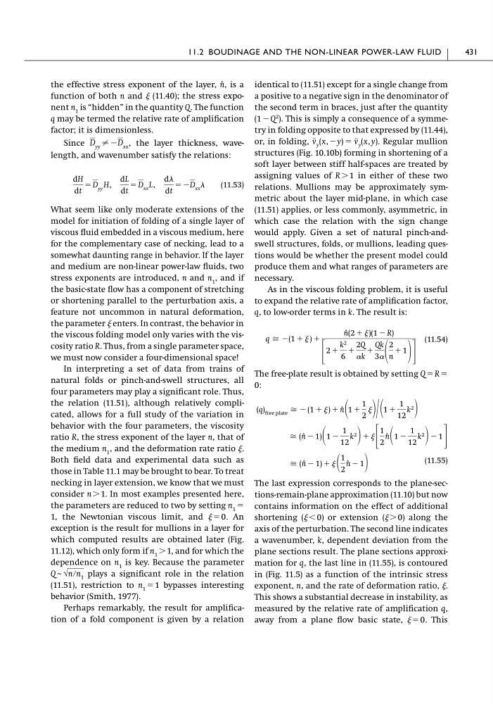
q, to low-order terms in k. The result is:
(11.54)
The free-plate result is obtained by setting Q ϭ R ϭ
0:
(11.55)
The last expression corresponds to the plane-sections-remain-plane approximation (11.10) but now
contains information on the effect of additional
shortening ( Ͻ 0) or extension ( Ͼ 0) along the
axis of the perturbation. The second line indicates
a wavenumber, k, dependent deviation from the
plane sections result. The plane sections approximation for q, the last line in (11.55), is contoured
in (Fig. 11.5) as a function of the intrinsic stress
exponent, n, and the rate of deformation ratio, .
This shows a substantial decrease in instability, as
measured by the relative rate of amplification q,
away from a plane flow basic state, ϭ 0. This
Х (n ˆ Ϫ 1) ϩ
1
2
n ˆ Ϫ 1
Х (n ˆ Ϫ 1) 1 Ϫ
1
12
k 2
ϩ ΄
1
2
n ˆ 1 Ϫ
1
12
k 2
Ϫ 1 ΅
(q) free plate Х Ϫ (1 ϩ ) ϩ n ˆ 1 ϩ
1
2
ր 1 ϩ
1
12
k 2
q Х Ϫ(1 ϩ ) ϩ
n ˆ(2 ϩ )(1 Ϫ R)
΄
2 ϩ
k 2
6
ϩ
2Q
␣k
ϩ
Qk
3␣
2
n
ϩ 1
΅
v ~ y (x, Ϫy) ϭ v ~ y (x, y).
11.2 BOUDINAGE AND THE NON-LINEAR POWER-LAW FLUID
431
is a
function of both n and (11.40); the stress exponent n 1 is “hidden” in the quantity Q. The function
q may be termed the relative rate of amplification
factor; it is dimensionless.
Since
the layer thickness, wavelength, and wavenumber satisfy the relations:
(11.53)
What seem like only moderate extensions of the
model for initiation of folding of a single layer of
viscous fluid embedded in a viscous medium, here
for the complementary case of necking, lead to a
somewhat daunting range in behavior. If the layer
and medium are non-linear power-law fluids, two
stress exponents are introduced, n and n 1 , and if
the basic-state flow has a component of stretching
or shortening parallel to the perturbation axis, a
feature not uncommon in natural deformation,
the parameter enters. In contrast, the behavior in
the viscous folding model only varies with the viscosity ratio R. Thus, from a single parameter space,
we must now consider a four-dimensional space!
In interpreting a set of data from trains of
natural folds or pinch-and-swell structures, all
four parameters may play a significant role. Thus,
the relation (11.51), although relatively complicated, allows for a full study of the variation in
behavior with the four parameters, the viscosity
ratio R, the stress exponent of the layer n, that of
the medium n 1 , and the deformation rate ratio .
Both field data and experimental data such as
those in Table 11.1 may be brought to bear. To treat
necking in layer extension, we know that we must
consider n Ͼ 1. In most examples presented here,
the parameters are reduced to two by setting n 1 ϭ
1, the Newtonian viscous limit, and ϭ 0. An
exception is the result for mullions in a layer for
which computed results are obtained later (Fig.
11.12), which only form if n 1 Ͼ 1, and for which the
dependence on n 1 is key. Because the parameter
plays a significant role in the relation
(11.51), restriction to n 1 ϭ 1 bypasses interesting
behavior (Smith, 1977).
Perhaps remarkably, the result for amplification of a fold component is given by a relation
Q ~ √nրn 1
dH
dt
ϭ D yy H,
dL
dt
ϭ D xx L,
d
dt
ϭ ϪD xx
D yy ϶ ϪD xx ,
n ˆ,
identical to (11.51) except for a single change from
a positive to a negative sign in the denominator of
the second term in braces, just after the quantity
(1 Ϫ Q
2 ). This is simply a consequence of a symmetry in folding opposite to that expressed by (11.44),
or, in folding,
Regular mullion
structures (Fig. 10.10b) forming in shortening of a
soft layer between stiff half-spaces are treated by
assigning values of R Ͼ 1 in either of these two
relations. Mullions may be approximately symmetric about the layer mid-plane, in which case
(11.51) applies, or less commonly, asymmetric, in
which case the relation with the sign change
would apply. Given a set of natural pinch-andswell structures, folds, or mullions, leading questions would be whether the present model could
produce them and what ranges of parameters are
necessary.
As in the viscous folding problem, it is useful
to expand the relative rate of amplification factor,
q, to low-order terms in k. The result is:
(11.54)
The free-plate result is obtained by setting Q ϭ R ϭ
0:
(11.55)
The last expression corresponds to the plane-sections-remain-plane approximation (11.10) but now
contains information on the effect of additional
shortening ( Ͻ 0) or extension ( Ͼ 0) along the
axis of the perturbation. The second line indicates
a wavenumber, k, dependent deviation from the
plane sections result. The plane sections approximation for q, the last line in (11.55), is contoured
in (Fig. 11.5) as a function of the intrinsic stress
exponent, n, and the rate of deformation ratio, .
This shows a substantial decrease in instability, as
measured by the relative rate of amplification q,
away from a plane flow basic state, ϭ 0. This
Х (n ˆ Ϫ 1) ϩ
1
2
n ˆ Ϫ 1
Х (n ˆ Ϫ 1) 1 Ϫ
1
12
k 2
ϩ ΄
1
2
n ˆ 1 Ϫ
1
12
k 2
Ϫ 1 ΅
(q) free plate Х Ϫ (1 ϩ ) ϩ n ˆ 1 ϩ
1
2
ր 1 ϩ
1
12
k 2
q Х Ϫ(1 ϩ ) ϩ
n ˆ(2 ϩ )(1 Ϫ R)
΄
2 ϩ
k 2
6
ϩ
2Q
␣k
ϩ
Qk
3␣
2
n
ϩ 1
΅
v ~ y (x, Ϫy) ϭ v ~ y (x, y).
11.2 BOUDINAGE AND THE NON-LINEAR POWER-LAW FLUID
431