

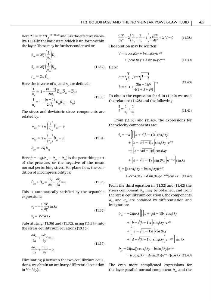
Here
and is the effective viscosity (11.14) in the basic state, which is uniform within
the layer. These may be further condensed to:
(11.32)
Here the inverse of n x and n y are defined:
(11.33)
The stress and deviatoric stress components are
related by:
(11.34)
Here
is the perturbing part
of the pressure, or the negative of the mean
normal perturbing stress. For plane flow, the condition of incompressibility is:
(11.35)
This is automatically satisfied by the separable
expressions:
(11.36)
Substituting (11.36) and (11.32), using (11.34), into
the stress equilibrium equations (10.15):
(11.37)
Eliminating between the two equilibrium equations, we obtain an ordinary differential equation
in V ϭ V(y):
p ~
Ѩ ~ xy
Ѩx
ϩ
Ѩ ~ yy
Ѩy
ϭ 0
Ѩ ~ xx
Ѩx
ϩ
Ѩ ~ xy
Ѩy
ϭ 0
v ~
x ϭ V cos x
v ~
x ϭ Ϫ
1
dV
dy
sin x
D
~
xx
ϩ D
~
yy
ϭ
Ѩv ~ x
Ѩx
ϩ
Ѩv ~ y
Ѩx
ϭ 0
p ~ ϭ Ϫ
1
3 ( ~ xx ϩ ~ yy ϩ ~ zz )
~
xy
Х 2 D
~
xy
~
yy
Х 2
1
n y
D
~
yy
Ϫ p ~
~
xx
Х 2
1
n x
D
~
xx
Ϫ p ~
1
n y
ϭ 1 ϩ
(n Ϫ 1)
2nI 2
D yy (D xx Ϫ D yy )
1
n x
Х 1 Ϫ
(n Ϫ 1)
2nI 2
D xx (D xx Ϫ D yy )
s ~
xy
Х 2 D
~
xy
s ~
yy
Х 2
1
n y
D
~
yy
s ~
xx
Х 2
1
n x D
~
xx
2 ϭ B Ϫ1րn I
Ϫ (nϪ1) ր2n
2
(11.38)
The solution may be written:
(11.39)
Here:
(11.40)
To obtain the expression for n ˆ in (11.40) we used
the relations (11.28) and the following:
(11.41)
From (11.36) and (11.40), the expressions for
the velocity components are:
(11.42)
From the third equation in (11.32) and (11.42) the
stress component
may be obtained, and from
the stress equilibrium equations, the components
and
are obtained by differentiation and
integration:
(11.43)
The even more complicated expressions for
the layer-parallel normal component
and the
~ xx
Ϫ (c cos y ϩ d sin y) e Ϫ␣y ] cos x
~ yy ϭ 2␣[(a cos y ϩ b sin y) e ␣y
ϩ ΄dϩ √ (n ˆ Ϫ 1)c΅ sin y · e Ϫ␣y ͡ sin x
ϩ Ά΄ c Ϫ √ (n ˆ Ϫ 1)d΅ cos y
ϩ ΄bϪ √ (n ˆ Ϫ 1)a΅sin y · e ␣y
~ xy ϭ Ϫ2␣ 2 ͠ Ά΄ a ϩ √ (n ˆ Ϫ 1)b΅ cos y
~ yy
~ xx
~ xy
ϩ (c cos y ϩ d sin y)e
Ϫ␣y ] cos x
v
~
y
ϭ [(a cos y ϩ b sin y)e
␣y
ϩ ΄dϩ √(n
^ Ϫ 1)c΅sin y · e Ϫ␣y ͡ sin x
Ϫ Ά΄ c Ϫ √(n
^ Ϫ 1)d΅cos y
ϩ ΄bϪ √(n
^ Ϫ 1) a΅sin y · e
␣y
v ~
x
ϭ Ϫ␣ ͠ Ά΄ a ϩ √(n
^ Ϫ 1)b΅cos y
2
n ˆ
ϭ
1
n x
ˇ
ϩ
1
n y
n ˆ ϭ n ΄
1 ϩ
3(n Ϫ 1) 2
4(1 ϩ ϩ 2 ) ΅
Ϫ1
␣ ϭ
√
1
n ˆ
,  ϭ
√
1 Ϫ
1
n ˆ
ϩ (c cos y ϩ d sin y)e ␣y
V ϭ (a cos y ϩ b sin y)e ␣y
d 4 V
dy 4 Ϫ 2
1
n x
ϩ
1
n y
Ϫ 1
2 d 2 V
dy 2 ϩ 4 V ϭ 0
11.2 BOUDINAGE AND THE NON-LINEAR POWER-LAW FLUID
429
and is the effective viscosity (11.14) in the basic state, which is uniform within
the layer. These may be further condensed to:
(11.32)
Here the inverse of n x and n y are defined:
(11.33)
The stress and deviatoric stress components are
related by:
(11.34)
Here
is the perturbing part
of the pressure, or the negative of the mean
normal perturbing stress. For plane flow, the condition of incompressibility is:
(11.35)
This is automatically satisfied by the separable
expressions:
(11.36)
Substituting (11.36) and (11.32), using (11.34), into
the stress equilibrium equations (10.15):
(11.37)
Eliminating between the two equilibrium equations, we obtain an ordinary differential equation
in V ϭ V(y):
p ~
Ѩ ~ xy
Ѩx
ϩ
Ѩ ~ yy
Ѩy
ϭ 0
Ѩ ~ xx
Ѩx
ϩ
Ѩ ~ xy
Ѩy
ϭ 0
v ~
x ϭ V cos x
v ~
x ϭ Ϫ
1
dV
dy
sin x
D
~
xx
ϩ D
~
yy
ϭ
Ѩv ~ x
Ѩx
ϩ
Ѩv ~ y
Ѩx
ϭ 0
p ~ ϭ Ϫ
1
3 ( ~ xx ϩ ~ yy ϩ ~ zz )
~
xy
Х 2 D
~
xy
~
yy
Х 2
1
n y
D
~
yy
Ϫ p ~
~
xx
Х 2
1
n x
D
~
xx
Ϫ p ~
1
n y
ϭ 1 ϩ
(n Ϫ 1)
2nI 2
D yy (D xx Ϫ D yy )
1
n x
Х 1 Ϫ
(n Ϫ 1)
2nI 2
D xx (D xx Ϫ D yy )
s ~
xy
Х 2 D
~
xy
s ~
yy
Х 2
1
n y
D
~
yy
s ~
xx
Х 2
1
n x D
~
xx
2 ϭ B Ϫ1րn I
Ϫ (nϪ1) ր2n
2
(11.38)
The solution may be written:
(11.39)
Here:
(11.40)
To obtain the expression for n ˆ in (11.40) we used
the relations (11.28) and the following:
(11.41)
From (11.36) and (11.40), the expressions for
the velocity components are:
(11.42)
From the third equation in (11.32) and (11.42) the
stress component
may be obtained, and from
the stress equilibrium equations, the components
and
are obtained by differentiation and
integration:
(11.43)
The even more complicated expressions for
the layer-parallel normal component
and the
~ xx
Ϫ (c cos y ϩ d sin y) e Ϫ␣y ] cos x
~ yy ϭ 2␣[(a cos y ϩ b sin y) e ␣y
ϩ ΄dϩ √ (n ˆ Ϫ 1)c΅ sin y · e Ϫ␣y ͡ sin x
ϩ Ά΄ c Ϫ √ (n ˆ Ϫ 1)d΅ cos y
ϩ ΄bϪ √ (n ˆ Ϫ 1)a΅sin y · e ␣y
~ xy ϭ Ϫ2␣ 2 ͠ Ά΄ a ϩ √ (n ˆ Ϫ 1)b΅ cos y
~ yy
~ xx
~ xy
ϩ (c cos y ϩ d sin y)e
Ϫ␣y ] cos x
v
~
y
ϭ [(a cos y ϩ b sin y)e
␣y
ϩ ΄dϩ √(n
^ Ϫ 1)c΅sin y · e Ϫ␣y ͡ sin x
Ϫ Ά΄ c Ϫ √(n
^ Ϫ 1)d΅cos y
ϩ ΄bϪ √(n
^ Ϫ 1) a΅sin y · e
␣y
v ~
x
ϭ Ϫ␣ ͠ Ά΄ a ϩ √(n
^ Ϫ 1)b΅cos y
2
n ˆ
ϭ
1
n x
ˇ
ϩ
1
n y
n ˆ ϭ n ΄
1 ϩ
3(n Ϫ 1) 2
4(1 ϩ ϩ 2 ) ΅
Ϫ1
␣ ϭ
√
1
n ˆ
,  ϭ
√
1 Ϫ
1
n ˆ
ϩ (c cos y ϩ d sin y)e ␣y
V ϭ (a cos y ϩ b sin y)e ␣y
d 4 V
dy 4 Ϫ 2
1
n x
ϩ
1
n y
Ϫ 1
2 d 2 V
dy 2 ϩ 4 V ϭ 0
11.2 BOUDINAGE AND THE NON-LINEAR POWER-LAW FLUID
429