

approximation to a layered medium made up of
alternating layers of stiff and soft isotropic
viscous fluid when the scale of the flow of interest
is much greater than the layer thickness, as in the
case of chevron folds. Suppose the layers have
thicknesses h 1 and h 2 and viscosities 1 and 2 , and
take the axes x and z parallel to layering so the yaxis is normal to the layering. The bulk properties
of this composite material are obtained as follows.
In layer-parallel extension, the rates of extension
in the two layer types must be equal. In the two inplane directions:
(10.159)
For simplicity, consider plane flow in the (x, y)plane, so that for example:
(10.160)
Then, developing the first of (10.159):
(10.161)
The components of normal stress acting normal
to the interface are equal. The last expression in
(10.161) identifies a bulk layer-parallel normal
stress xx and a bulk viscosity in layer-parallel
shortening or extension n . The bulk normal
stress component parallel to the layering is:
(10.162)
Combining (10.161) and (10.162):
(10.163)
Here f 1 and f 2 are the thickness (volume) fractions
of the alternating layer types. The bulk viscosity in
layer-parallel shear is obtained by taking the
average of the rate of shear:
(10.164)
Rearranging, the bulk viscosity in layer-parallel
shear is:
D xy ϭ f 1 D (1)
xy ϩ f 2 D (2)
xy ϭ f 1
xy
2 1 ϩ f 2
xy
2 2 ϭ
xy
2 s
n ϭ
h 1 1 ϩ h 2 2
h 1 ϩ h 2
ϭ f 1 1 ϩ f 2 2
xx ϭ
h 1 (1)
xx ϩ h 2 (2)
xx
h 1 ϩ h 2
( (1)
xx Ϫ yy ) ր4 1 ϭ ( (2)
xx Ϫ yy ) ր4 2 ϭ ( xx Ϫ yy ) ր4 n
(1)
zz ϭ ( (1)
xx ϩ yy ) ր2
D (1)
zz ϭ ΄ (1)
zz Ϫ
1
3 ( (1)
xx ϩ yy ϩ (1)
zz )΅ ր 2 1 ϭ 0
D (1)
xx ϭ D (2)
xx ϭ D xx , D (1)
zz ϭ D (2)
zz ϭ D zz
(10.165)
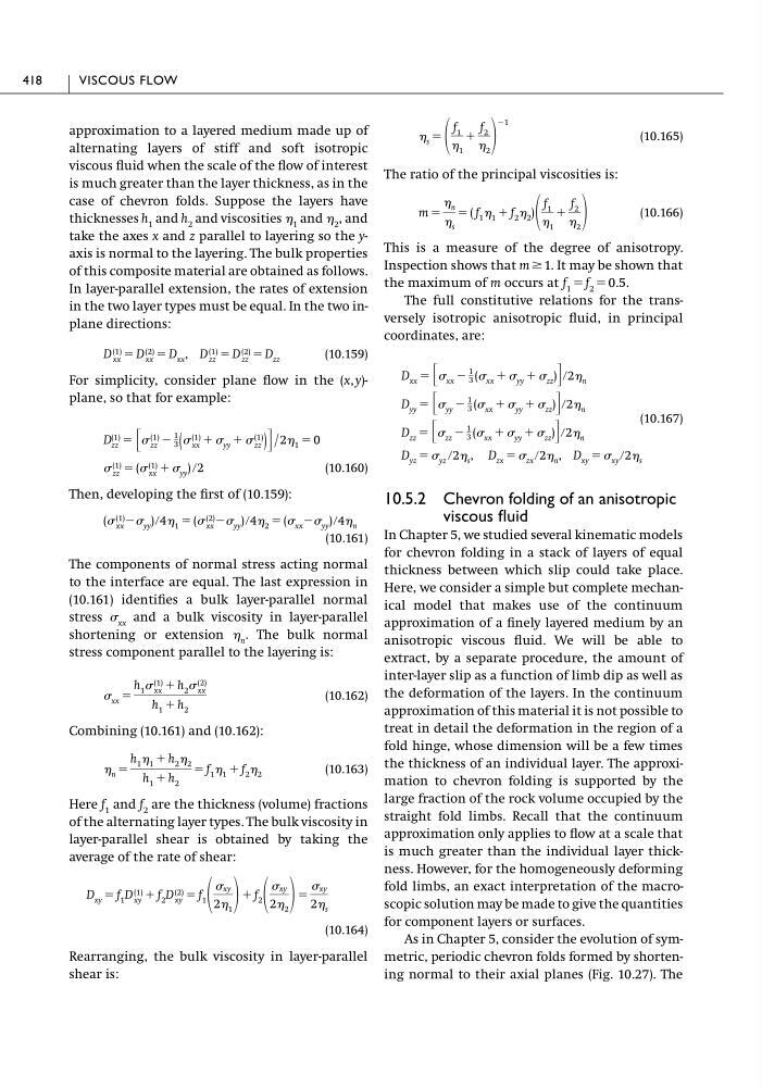
The ratio of the principal viscosities is:
(10.166)
This is a measure of the degree of anisotropy.
Inspection shows that m Ն 1. It may be shown that
the maximum of m occurs at f 1 ϭ f 2 ϭ 0.5.
The full constitutive relations for the transversely isotropic anisotropic fluid, in principal
coordinates, are:
(10.167)
10.5.2 Chevron folding of an anisotropic
viscous fluid
In Chapter 5, we studied several kinematic models
for chevron folding in a stack of layers of equal
thickness between which slip could take place.
Here, we consider a simple but complete mechanical model that makes use of the continuum
approximation of a finely layered medium by an
anisotropic viscous fluid. We will be able to
extract, by a separate procedure, the amount of
inter-layer slip as a function of limb dip as well as
the deformation of the layers. In the continuum
approximation of this material it is not possible to
treat in detail the deformation in the region of a
fold hinge, whose dimension will be a few times
the thickness of an individual layer. The approximation to chevron folding is supported by the
large fraction of the rock volume occupied by the
straight fold limbs. Recall that the continuum
approximation only applies to flow at a scale that
is much greater than the individual layer thickness. However, for the homogeneously deforming
fold limbs, an exact interpretation of the macroscopic solution may be made to give the quantities
for component layers or surfaces.
As in Chapter 5, consider the evolution of symmetric, periodic chevron folds formed by shortening normal to their axial planes (Fig. 10.27). The
D yz ϭ yz ր2 s , D zx ϭ zx ր2 n , D xy ϭ xy ր2 s
D zz ϭ ΄ zz Ϫ
1
3 ( xx ϩ yy ϩ zz )΅ր2 n
D yy ϭ ΄ yy Ϫ
1
3 ( xx ϩ yy ϩ zz )΅ր2 n
D xx ϭ ΄ xx Ϫ
1
3 ( xx ϩ yy ϩ zz )΅ր2 n
m ϭ
n
s
ϭ ( f 1 1 ϩ f 2 2 )
f 1
1
ϩ
f 2
2
s ϭ
f 1
1
ϩ
f 2
2
Ϫ1
418
VISCOUS FLOW
alternating layers of stiff and soft isotropic
viscous fluid when the scale of the flow of interest
is much greater than the layer thickness, as in the
case of chevron folds. Suppose the layers have
thicknesses h 1 and h 2 and viscosities 1 and 2 , and
take the axes x and z parallel to layering so the yaxis is normal to the layering. The bulk properties
of this composite material are obtained as follows.
In layer-parallel extension, the rates of extension
in the two layer types must be equal. In the two inplane directions:
(10.159)
For simplicity, consider plane flow in the (x, y)plane, so that for example:
(10.160)
Then, developing the first of (10.159):
(10.161)
The components of normal stress acting normal
to the interface are equal. The last expression in
(10.161) identifies a bulk layer-parallel normal
stress xx and a bulk viscosity in layer-parallel
shortening or extension n . The bulk normal
stress component parallel to the layering is:
(10.162)
Combining (10.161) and (10.162):
(10.163)
Here f 1 and f 2 are the thickness (volume) fractions
of the alternating layer types. The bulk viscosity in
layer-parallel shear is obtained by taking the
average of the rate of shear:
(10.164)
Rearranging, the bulk viscosity in layer-parallel
shear is:
D xy ϭ f 1 D (1)
xy ϩ f 2 D (2)
xy ϭ f 1
xy
2 1 ϩ f 2
xy
2 2 ϭ
xy
2 s
n ϭ
h 1 1 ϩ h 2 2
h 1 ϩ h 2
ϭ f 1 1 ϩ f 2 2
xx ϭ
h 1 (1)
xx ϩ h 2 (2)
xx
h 1 ϩ h 2
( (1)
xx Ϫ yy ) ր4 1 ϭ ( (2)
xx Ϫ yy ) ր4 2 ϭ ( xx Ϫ yy ) ր4 n
(1)
zz ϭ ( (1)
xx ϩ yy ) ր2
D (1)
zz ϭ ΄ (1)
zz Ϫ
1
3 ( (1)
xx ϩ yy ϩ (1)
zz )΅ ր 2 1 ϭ 0
D (1)
xx ϭ D (2)
xx ϭ D xx , D (1)
zz ϭ D (2)
zz ϭ D zz
(10.165)
The ratio of the principal viscosities is:
(10.166)
This is a measure of the degree of anisotropy.
Inspection shows that m Ն 1. It may be shown that
the maximum of m occurs at f 1 ϭ f 2 ϭ 0.5.
The full constitutive relations for the transversely isotropic anisotropic fluid, in principal
coordinates, are:
(10.167)
10.5.2 Chevron folding of an anisotropic
viscous fluid
In Chapter 5, we studied several kinematic models
for chevron folding in a stack of layers of equal
thickness between which slip could take place.
Here, we consider a simple but complete mechanical model that makes use of the continuum
approximation of a finely layered medium by an
anisotropic viscous fluid. We will be able to
extract, by a separate procedure, the amount of
inter-layer slip as a function of limb dip as well as
the deformation of the layers. In the continuum
approximation of this material it is not possible to
treat in detail the deformation in the region of a
fold hinge, whose dimension will be a few times
the thickness of an individual layer. The approximation to chevron folding is supported by the
large fraction of the rock volume occupied by the
straight fold limbs. Recall that the continuum
approximation only applies to flow at a scale that
is much greater than the individual layer thickness. However, for the homogeneously deforming
fold limbs, an exact interpretation of the macroscopic solution may be made to give the quantities
for component layers or surfaces.
As in Chapter 5, consider the evolution of symmetric, periodic chevron folds formed by shortening normal to their axial planes (Fig. 10.27). The
D yz ϭ yz ր2 s , D zx ϭ zx ր2 n , D xy ϭ xy ր2 s
D zz ϭ ΄ zz Ϫ
1
3 ( xx ϩ yy ϩ zz )΅ր2 n
D yy ϭ ΄ yy Ϫ
1
3 ( xx ϩ yy ϩ zz )΅ր2 n
D xx ϭ ΄ xx Ϫ
1
3 ( xx ϩ yy ϩ zz )΅ր2 n
m ϭ
n
s
ϭ ( f 1 1 ϩ f 2 2 )
f 1
1
ϩ
f 2
2
s ϭ
f 1
1
ϩ
f 2
2
Ϫ1
418
VISCOUS FLOW