

Using the Olympic accretionary wedge as an
example (Fig. 10.8a), we may roughly estimate the
model parameters (Batt et al., 2001; Brandon,
2004). A rate of erosion Ϸ1 km Ma
Ϫ1 is associated
with a topographic amplitude A Ϸ 1.5 km, giving
an erosion constant K Ϸ 2/3 Ma
Ϫ1 . Using a density
Ϸ 2700 kg m
Ϫ3 , acceleration of gravity g ϭ 9.8 m
s
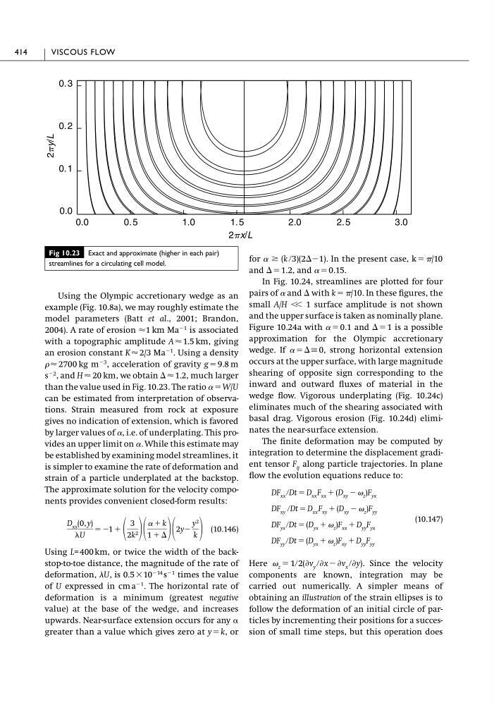
Ϫ2 , and H Ϸ 20 km, we obtain ⌬ Ϸ 1.2, much larger
than the value used in Fig. 10.23. The ratio ␣ ϭ W/U
can be estimated from interpretation of observations. Strain measured from rock at exposure
gives no indication of extension, which is favored
by larger values of ␣, i.e. of underplating. This provides an upper limit on ␣. While this estimate may
be established by examining model streamlines, it
is simpler to examine the rate of deformation and
strain of a particle underplated at the backstop.
The approximate solution for the velocity components provides convenient closed-form results:
(10.146)
Using L= 400 km, or twice the width of the backstop-to-toe distance, the magnitude of the rate of
deformation, U, is 0.5 ϫ10
Ϫ14 s
Ϫ1 times the value
of U expressed in cm a
Ϫ1 . The horizontal rate of
deformation is a minimum (greatest negative
value) at the base of the wedge, and increases
upwards. Near-surface extension occurs for any ␣
greater than a value which gives zero at y ϭ k, or
D xx (0, y)
U
ϭ Ϫ1 ϩ
3
2k 2
␣ ϩ k
1 ϩ ⌬
2yϪ
y 2
k
for
In the present case, k ϭ /10
and ⌬ϭ1.2, and ␣ ϭ 0.15.
In Fig. 10.24, streamlines are plotted for four
pairs of ␣ and ⌬ with k ϭ /10. In these figures, the
small A/H Ͻ Ͻ 1 surface amplitude is not shown
and the upper surface is taken as nominally plane.
Figure 10.24a with ␣ ϭ 0.1 and ⌬ϭ1 is a possible
approximation for the Olympic accretionary
wedge. If ␣ ϭ⌬ഡ0, strong horizontal extension
occurs at the upper surface, with large magnitude
shearing of opposite sign corresponding to the
inward and outward fluxes of material in the
wedge flow. Vigorous underplating (Fig. 10.24c)
eliminates much of the shearing associated with
basal drag. Vigorous erosion (Fig. 10.24d) eliminates the near-surface extension.
The finite deformation may be computed by
integration to determine the displacement gradient tensor F ij along particle trajectories. In plane
flow the evolution equations reduce to:
(10.147)
Here
Since the velocity
components are known, integration may be
carried out numerically. A simpler means of
obtaining an illustration of the strain ellipses is to
follow the deformation of an initial circle of particles by incrementing their positions for a succession of small time steps, but this operation does
z ϭ 1ր2(Ѩv y րѨx Ϫ Ѩv x րѨy).
DF yy րDt ϭ (D yx ϩ z )F xy ϩ D yy F yy
DF yx րDt ϭ (D yx ϩ z )F xx ϩ D yy F yx
DF xy րDt ϭ D xx F xy ϩ (D xy Ϫ z )F yy
DF xx րDt ϭ D xx F xx ϩ (D xy Ϫ z )F yx
␣ Ն (k ր3)(2⌬Ϫ1).
414
VISCOUS FLOW
Fig 10.23 Exact and approximate (higher in each pair)
streamlines for a circulating cell model.
0.0
0. 5
1.0
1. 5
2.0
2. 5
3.0
0.0
0. 1
0. 2
0. 3
2py/L
2px/L
example (Fig. 10.8a), we may roughly estimate the
model parameters (Batt et al., 2001; Brandon,
2004). A rate of erosion Ϸ1 km Ma
Ϫ1 is associated
with a topographic amplitude A Ϸ 1.5 km, giving
an erosion constant K Ϸ 2/3 Ma
Ϫ1 . Using a density
Ϸ 2700 kg m
Ϫ3 , acceleration of gravity g ϭ 9.8 m
s
Ϫ2 , and H Ϸ 20 km, we obtain ⌬ Ϸ 1.2, much larger
than the value used in Fig. 10.23. The ratio ␣ ϭ W/U
can be estimated from interpretation of observations. Strain measured from rock at exposure
gives no indication of extension, which is favored
by larger values of ␣, i.e. of underplating. This provides an upper limit on ␣. While this estimate may
be established by examining model streamlines, it
is simpler to examine the rate of deformation and
strain of a particle underplated at the backstop.
The approximate solution for the velocity components provides convenient closed-form results:
(10.146)
Using L= 400 km, or twice the width of the backstop-to-toe distance, the magnitude of the rate of
deformation, U, is 0.5 ϫ10
Ϫ14 s
Ϫ1 times the value
of U expressed in cm a
Ϫ1 . The horizontal rate of
deformation is a minimum (greatest negative
value) at the base of the wedge, and increases
upwards. Near-surface extension occurs for any ␣
greater than a value which gives zero at y ϭ k, or
D xx (0, y)
U
ϭ Ϫ1 ϩ
3
2k 2
␣ ϩ k
1 ϩ ⌬
2yϪ
y 2
k
for
In the present case, k ϭ /10
and ⌬ϭ1.2, and ␣ ϭ 0.15.
In Fig. 10.24, streamlines are plotted for four
pairs of ␣ and ⌬ with k ϭ /10. In these figures, the
small A/H Ͻ Ͻ 1 surface amplitude is not shown
and the upper surface is taken as nominally plane.
Figure 10.24a with ␣ ϭ 0.1 and ⌬ϭ1 is a possible
approximation for the Olympic accretionary
wedge. If ␣ ϭ⌬ഡ0, strong horizontal extension
occurs at the upper surface, with large magnitude
shearing of opposite sign corresponding to the
inward and outward fluxes of material in the
wedge flow. Vigorous underplating (Fig. 10.24c)
eliminates much of the shearing associated with
basal drag. Vigorous erosion (Fig. 10.24d) eliminates the near-surface extension.
The finite deformation may be computed by
integration to determine the displacement gradient tensor F ij along particle trajectories. In plane
flow the evolution equations reduce to:
(10.147)
Here
Since the velocity
components are known, integration may be
carried out numerically. A simpler means of
obtaining an illustration of the strain ellipses is to
follow the deformation of an initial circle of particles by incrementing their positions for a succession of small time steps, but this operation does
z ϭ 1ր2(Ѩv y րѨx Ϫ Ѩv x րѨy).
DF yy րDt ϭ (D yx ϩ z )F xy ϩ D yy F yy
DF yx րDt ϭ (D yx ϩ z )F xx ϩ D yy F yx
DF xy րDt ϭ D xx F xy ϩ (D xy Ϫ z )F yy
DF xx րDt ϭ D xx F xx ϩ (D xy Ϫ z )F yx
␣ Ն (k ր3)(2⌬Ϫ1).
414
VISCOUS FLOW
Fig 10.23 Exact and approximate (higher in each pair)
streamlines for a circulating cell model.
0.0
0. 5
1.0
1. 5
2.0
2. 5
3.0
0.0
0. 1
0. 2
0. 3
2py/L
2px/L